import numpy as np
import pandas as pd
from sklearn.datasets import make_regression
from sklearn.linear_model import LinearRegression
from sklearn.linear_model import Lasso
from sklearn.linear_model import Ridge
from sklearn.linear_model import ElasticNet
from sklearn.preprocessing import StandardScalerCS 307: Week 05
Regularization
# create some data
X, y = make_regression(n_samples=100, n_features=20, noise=0.1, random_state=42)
# view first two rows of the X data
X[0:2]array([[-0.92216532, 1.87679581, 0.75698862, 0.27996863, 0.72576662,
0.48100923, 1.35563786, -1.2446547 , 0.4134349 , 0.86960592,
0.65436566, -1.12548905, 2.44575198, 0.12922118, 0.22388402,
1.49604431, -0.7737892 , -0.05558467, 0.10939479, -1.77872025],
[-0.08310557, -1.4575515 , -1.40631746, -0.1601328 , -0.79602586,
1.07600714, 0.76005596, -0.75215641, 0.08243975, -1.50472037,
-1.87517247, 0.67134008, 0.21319663, -0.75196933, 0.02131165,
1.34045045, -0.30920908, 0.11502608, -0.31905394, 0.31917451]])# view some examples from the y data
y[0:5]array([ 108.81742028, -250.567936 , 1.86765761, 127.84318259,
34.15127975])# get a better look at the X data by temporarily displaying it as a pandas data frame
pd.DataFrame(X)| 0 | 1 | 2 | 3 | 4 | 5 | 6 | 7 | 8 | 9 | 10 | 11 | 12 | 13 | 14 | 15 | 16 | 17 | 18 | 19 | |
|---|---|---|---|---|---|---|---|---|---|---|---|---|---|---|---|---|---|---|---|---|
| 0 | -0.922165 | 1.876796 | 0.756989 | 0.279969 | 0.725767 | 0.481009 | 1.355638 | -1.244655 | 0.413435 | 0.869606 | 0.654366 | -1.125489 | 2.445752 | 0.129221 | 0.223884 | 1.496044 | -0.773789 | -0.055585 | 0.109395 | -1.778720 |
| 1 | -0.083106 | -1.457551 | -1.406317 | -0.160133 | -0.796026 | 1.076007 | 0.760056 | -0.752156 | 0.082440 | -1.504720 | -1.875172 | 0.671340 | 0.213197 | -0.751969 | 0.021312 | 1.340450 | -0.309209 | 0.115026 | -0.319054 | 0.319175 |
| 2 | 0.810808 | -1.662492 | -0.134309 | -0.308034 | -0.209222 | -1.683438 | -1.748532 | 1.126705 | 1.304340 | 0.793489 | -1.105705 | 0.779661 | 1.310309 | 1.395684 | -0.805870 | -0.410814 | 1.032546 | -0.214921 | -0.562168 | -1.090966 |
| 3 | 0.536653 | -0.756795 | -1.046911 | 0.455888 | 0.268592 | 1.528468 | 0.718953 | 1.501334 | 0.996048 | 1.185704 | 1.328194 | 2.165002 | -0.643518 | 0.927840 | 0.507836 | -0.250833 | -1.421811 | 0.556230 | 0.057013 | -0.322680 |
| 4 | 1.532739 | -0.401220 | 0.519347 | 1.451144 | 0.183342 | 2.189803 | 0.401712 | 0.012592 | 0.690144 | -0.108760 | 0.024510 | 0.959271 | 2.153182 | -0.767348 | -0.808298 | -0.773010 | 0.224092 | 0.497998 | 0.872321 | 0.097676 |
| ... | ... | ... | ... | ... | ... | ... | ... | ... | ... | ... | ... | ... | ... | ... | ... | ... | ... | ... | ... | ... |
| 95 | -0.114736 | -0.334501 | -0.792521 | 2.122156 | -0.707669 | 0.443819 | 0.865755 | -0.653329 | -1.200296 | 0.504987 | -1.260884 | 1.032465 | -1.519370 | -0.484234 | 0.774634 | 0.404982 | -0.474945 | 0.917862 | 1.266911 | 1.765454 |
| 96 | -0.599375 | 0.622850 | -1.594428 | -1.534114 | 0.115675 | 1.179297 | 0.046981 | -0.142379 | -0.450065 | 0.005244 | 0.711615 | 1.277677 | 0.332314 | -0.748487 | 0.067518 | 0.514439 | -1.067620 | -1.124642 | 1.551152 | 0.120296 |
| 97 | -0.152470 | -1.331233 | 0.133541 | -0.006071 | -0.290275 | 0.267392 | 0.956702 | 0.507991 | -0.785989 | 0.708109 | 0.388579 | 0.838491 | 0.081829 | -0.098890 | 0.321698 | -2.152891 | -1.836205 | 2.493000 | 0.919076 | -1.103367 |
| 98 | -1.379618 | 0.513085 | -0.971657 | 1.188913 | -0.881875 | -0.163067 | 0.862393 | 0.516178 | 0.953125 | -0.626717 | 0.800410 | 0.708304 | 0.351448 | 1.070150 | -0.744903 | 0.431923 | 0.725096 | 0.754291 | -0.026521 | -0.641482 |
| 99 | -2.848543 | -1.119670 | 0.771699 | 0.076822 | -0.428115 | 1.500760 | -1.739714 | 1.160827 | -0.362441 | 1.148766 | -0.046921 | -1.282992 | 0.996267 | -0.493757 | 0.850222 | 0.346504 | -1.294681 | 0.477041 | -1.556582 | -0.467701 |
100 rows × 20 columns
# create different linear models (some with regularization!)
linear = LinearRegression()
lasso = Lasso(alpha=0.1)
ridge = Ridge(alpha=0.1)
Relevant documentation:
# fit the models
linear.fit(X, y)
lasso.fit(X, y)
ridge.fit(X, y)Ridge(alpha=0.1)In a Jupyter environment, please rerun this cell to show the HTML representation or trust the notebook.
On GitHub, the HTML representation is unable to render, please try loading this page with nbviewer.org.
Ridge(alpha=0.1)
linear.coef_array([ 6.59316802e+00, 9.47572840e+01, 4.07080537e+01, -1.36954387e-03,
9.32945665e-03, -1.55281734e-02, 1.11188043e+01, 9.55121723e+01,
8.08254906e+01, 3.48859900e+01, 1.62428940e-02, 1.09659676e-02,
9.76125777e-03, 1.02690177e-02, -6.11540038e-03, 2.99366631e+01,
7.23584909e+00, 9.68705480e-03, -1.93391406e-03, 5.22797071e+01])ridge.coef_array([ 6.59850269e+00, 9.46618846e+01, 4.06454457e+01, 4.37714102e-03,
6.54059913e-03, -1.06479513e-02, 1.11069896e+01, 9.53732188e+01,
8.07112840e+01, 3.48957311e+01, 4.45154929e-04, 3.57365603e-02,
3.00167738e-02, 5.40170250e-03, -1.88067055e-02, 2.98957936e+01,
7.23859203e+00, -2.66565706e-02, -3.45743780e-02, 5.21972230e+01])lasso.coef_array([ 6.45386948, 94.67737779, 40.55794675, 0. , -0. ,
-0. , 10.98839003, 95.40225582, 80.67610577, 34.83198456,
-0. , 0. , 0. , -0. , -0. ,
29.82848069, 7.12581798, -0. , 0. , 52.17111821])lasso.coef_ / linear.coef_array([ 0.97887229, 0.99915673, 0.9963126 , -0. , -0. ,
0. , 0.98827084, 0.99884919, 0.99815176, 0.99845194,
-0. , 0. , 0. , -0. , 0. ,
0.99638629, 0.98479362, -0. , -0. , 0.99792292])lasso_0 = Lasso(alpha=0)
lasso_0.fit(X, y)/Library/Frameworks/Python.framework/Versions/3.11/lib/python3.11/site-packages/sklearn/base.py:1151: UserWarning: With alpha=0, this algorithm does not converge well. You are advised to use the LinearRegression estimator
return fit_method(estimator, *args, **kwargs)
/Library/Frameworks/Python.framework/Versions/3.11/lib/python3.11/site-packages/sklearn/linear_model/_coordinate_descent.py:628: UserWarning: Coordinate descent with no regularization may lead to unexpected results and is discouraged.
model = cd_fast.enet_coordinate_descent(Lasso(alpha=0)In a Jupyter environment, please rerun this cell to show the HTML representation or trust the notebook.
On GitHub, the HTML representation is unable to render, please try loading this page with nbviewer.org.
Lasso(alpha=0)
lasso_0.coef_array([ 6.59220650e+00, 9.47578704e+01, 4.07086530e+01, 1.67942913e-03,
7.04365608e-03, -1.08366993e-02, 1.11190745e+01, 9.55172343e+01,
8.08290446e+01, 3.48823135e+01, 1.51450701e-02, 6.76300320e-03,
6.58339664e-03, 1.01400600e-02, -4.48418689e-03, 2.99366761e+01,
7.23587178e+00, 1.20404224e-02, 6.35862604e-04, 5.22790377e+01])lasso_01 = Lasso(alpha=0.1)
lasso_05 = Lasso(alpha=5)lasso_01.fit(X, y)
lasso_05.fit(X, y)Lasso(alpha=5)In a Jupyter environment, please rerun this cell to show the HTML representation or trust the notebook.
On GitHub, the HTML representation is unable to render, please try loading this page with nbviewer.org.
Lasso(alpha=5)
lasso_01.coef_array([ 6.45386948, 94.67737779, 40.55794675, 0. , -0. ,
-0. , 10.98839003, 95.40225582, 80.67610577, 34.83198456,
-0. , 0. , 0. , -0. , -0. ,
29.82848069, 7.12581798, -0. , 0. , 52.17111821])lasso_05.coef_array([ 0. , 90.82037065, 33.18439832, 0. , -0. ,
-0. , 4.90698647, 90.05810943, 73.22163014, 32.39510376,
-0. , 0. , 0. , -0. , 0. ,
24.45096119, 1.92062117, -0. , 0. , 46.96663538])scaler = StandardScaler()
scaler.fit(X)
X_scaled = scaler.transform(X)np.mean(X, axis=0)array([ 0.06648265, -0.09066858, 0.14879335, -0.0092515 , 0.06688254,
0.13867757, -0.020263 , 0.1355665 , 0.04824566, 0.02152732,
-0.06736594, 0.11621231, 0.18151189, -0.02125737, 0.14082977,
0.16464492, -0.08393592, 0.01139174, -0.01378138, -0.0325596 ])np.mean(X_scaled, axis=0)array([-4.44089210e-17, -4.21884749e-17, -2.55351296e-17, -1.84574578e-17,
9.99200722e-18, 3.99680289e-17, -5.10702591e-17, -4.66293670e-17,
-8.38218384e-17, 2.22044605e-18, -3.92047506e-18, 4.44089210e-17,
3.66373598e-17, 3.21964677e-17, -3.44169138e-17, 2.35922393e-17,
-4.44089210e-18, 2.55351296e-17, 5.77315973e-17, 3.38618023e-17])np.std(X, axis=0)array([1.02482769, 0.97262509, 0.92892846, 0.89105338, 0.92304624,
0.91902508, 0.97366298, 0.94131669, 0.89996273, 1.07352597,
0.84522696, 1.01952759, 1.04023857, 1.04776952, 0.91703382,
1.08312224, 1.05773266, 1.1802187 , 1.00197408, 0.88057435])np.std(X_scaled, axis=0)array([1., 1., 1., 1., 1., 1., 1., 1., 1., 1., 1., 1., 1., 1., 1., 1., 1.,
1., 1., 1.])lasso.fit(X_scaled, y)Lasso(alpha=0.1)In a Jupyter environment, please rerun this cell to show the HTML representation or trust the notebook.
On GitHub, the HTML representation is unable to render, please try loading this page with nbviewer.org.
Lasso(alpha=0.1)
lasso.predict(X) # WRONG
lasso.predict(X_scaled) # correct
array([ 108.56929274, -250.27007327, 1.74711702, 127.74731283,
34.16484902, 6.73089519, -47.99671007, -323.75282966,
40.71830457, 12.39299331, -233.2758167 , -68.89474373,
-95.14530018, 55.75266526, -25.81229695, 77.54586244,
88.98514129, -200.10765794, 49.19701855, 421.46438405,
157.23398526, 87.67924179, -36.15995542, 216.57697103,
340.00532386, -275.91290738, 257.12555842, -374.03964729,
357.20158352, -244.88762318, 93.67700784, -39.95057358,
61.98410136, 212.02109074, 265.26394524, 281.77244047,
318.53883286, 28.62306877, -22.37384227, 234.1955855 ,
-238.8564661 , 280.59818363, -49.02400195, -89.68866067,
-60.59043932, 34.04378327, 147.98817117, 243.56423325,
-14.29619749, 79.54075017, -45.42211395, -36.5241835 ,
29.71181164, -176.91121525, 96.89249288, 52.16684761,
114.5794129 , -333.86642314, 226.29054183, -106.73890637,
-6.6769494 , 162.63925058, -30.94403975, -21.76185466,
-19.87450714, -227.84122694, 87.90333805, 11.65702773,
209.70645989, 214.75616587, -108.581903 , 199.07494731,
-130.09302298, 33.6694303 , -58.72737906, -100.74761299,
-254.15146038, -9.07234502, 157.97000597, -444.49241247,
6.22181382, -1.07204728, 59.76748702, -58.99329766,
-71.9214518 , 207.05877426, -20.81839889, -265.38705602,
97.88748469, 114.24112507, 144.72937082, -55.47105068,
86.01322255, 300.68411823, 22.14183285, -95.77237868,
-44.71399397, -236.20063655, 98.68319317, -13.91650175])Ensemble Methods
import numpy as np
from sklearn.datasets import make_regression
from sklearn.tree import DecisionTreeRegressor
import matplotlib.pyplot as plt
X, y = make_regression(n_samples=100, n_features=5, noise=0.3, random_state=42)dt = DecisionTreeRegressor(max_depth=3)
dt.fit(X, y)DecisionTreeRegressor(max_depth=3)In a Jupyter environment, please rerun this cell to show the HTML representation or trust the notebook.
On GitHub, the HTML representation is unable to render, please try loading this page with nbviewer.org.
DecisionTreeRegressor(max_depth=3)
preds = dt.predict(X)np.sqrt(np.mean((y - preds) ** 2))72.97884422360983# setup figure
fig, (ax) = plt.subplots(1, 1)
fig.set_size_inches(5, 5)
fig.set_dpi(100)
# add overall title
fig.suptitle('Predicted versus Actual')
# create subplot for linear model
ax.scatter(y, preds, color="dodgerblue")
ax.set_xlabel("Actual")
ax.set_ylabel("Predicted")
ax.grid(True, linestyle='--', color='lightgrey')
ax.axline((0, 0), slope=1, color="black")
# shot plot
plt.show()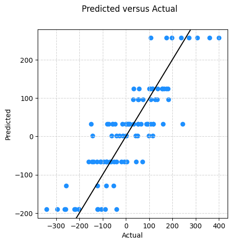
from sklearn.ensemble import RandomForestRegressor
from sklearn.ensemble import GradientBoostingRegressor
bagged = RandomForestRegressor(max_features=5)
rf = RandomForestRegressor(max_features=2)
boost = GradientBoostingRegressor()bagged.fit(X, y)
rf.fit(X, y)
boost.fit(X, y)GradientBoostingRegressor()In a Jupyter environment, please rerun this cell to show the HTML representation or trust the notebook.
On GitHub, the HTML representation is unable to render, please try loading this page with nbviewer.org.
GradientBoostingRegressor()
preds_dt = dt.predict(X)
preds_bagged = bagged.predict(X)
preds_rf = rf.predict(X)
preds_boost = boost.predict(X)
# setup figure
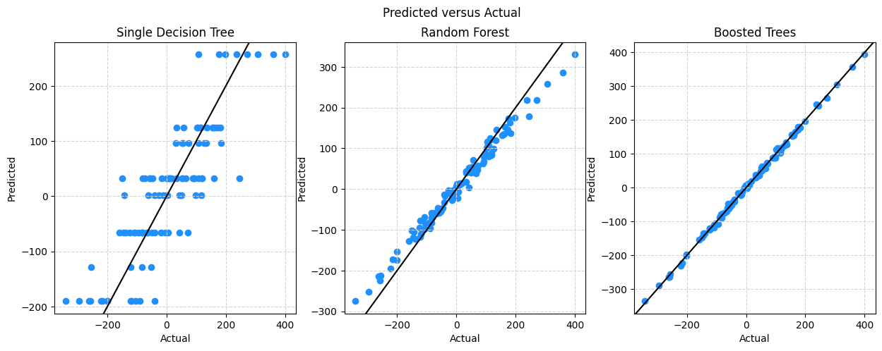
fig, (ax1, ax2, ax3) = plt.subplots(1, 3)
fig.set_size_inches(15, 5)
fig.set_dpi(100)
# add overall title
fig.suptitle('Predicted versus Actual')
# create subplot for dt
ax1.set_title("Single Decision Tree")
ax1.scatter(y, preds_dt, color="dodgerblue")
ax1.set_xlabel("Actual")
ax1.set_ylabel("Predicted")
ax1.grid(True, linestyle='--', color='lightgrey')
ax1.axline((0, 0), slope=1, color="black")
# create subplot for rf
ax2.set_title("Random Forest")
ax2.scatter(y, preds_rf, color="dodgerblue")
ax2.set_xlabel("Actual")
ax2.set_ylabel("Predicted")
ax2.grid(True, linestyle='--', color='lightgrey')
ax2.axline((0, 0), slope=1, color="black")
# create subplot for boost
ax3.set_title("Boosted Trees")
ax3.scatter(y, preds_boost, color="dodgerblue")
ax3.set_xlabel("Actual")
ax3.set_ylabel("Predicted")
ax3.grid(True, linestyle='--', color='lightgrey')
ax3.axline((0, 0), slope=1, color="black")
# shot plot
plt.show()