CS 307: Week 09

# Basics
import numpy as np
import pandas as pd
import matplotlib.pyplot as plt
import seaborn as sns

# Machine Learning
from sklearn.datasets import make_classification, load_breast_cancer
from sklearn.model_selection import train_test_split, GridSearchCV
from sklearn.preprocessing import StandardScaler
from sklearn.pipeline import Pipeline
from sklearn.ensemble import RandomForestClassifier
from sklearn.dummy import DummyClassifier
from sklearn.linear_model import LogisticRegression, LogisticRegressionCV

# Binary Classification
from sklearn.metrics import accuracy_score, confusion_matrix, classification_report, make_scorer
from sklearn.metrics import ConfusionMatrixDisplay
from sklearn.metrics import accuracy_score, recall_score, precision_score, f1_score, balanced_accuracy_score

Logistic Regression

X_train, y_train = make_classification(n_samples=250, n_features=5)
X_test, y_test = make_classification(n_samples=100, n_features=5)

y_train

array([0, 1, 0, 0, 0, 0, 0, 1, 0, 0, 1, 1, 0, 1, 0, 0, 1, 0, 1, 0, 0, 1,
       1, 1, 0, 0, 1, 0, 1, 1, 0, 1, 1, 0, 0, 1, 0, 1, 0, 1, 0, 1, 1, 1,
       1, 1, 1, 0, 1, 0, 1, 0, 1, 1, 1, 0, 1, 0, 1, 1, 1, 0, 1, 0, 1, 1,
       0, 1, 0, 0, 0, 1, 0, 1, 0, 1, 1, 0, 0, 1, 0, 1, 1, 1, 1, 1, 0, 1,
       1, 1, 0, 0, 1, 0, 0, 1, 1, 0, 0, 0, 1, 1, 1, 1, 0, 0, 0, 0, 0, 0,
       1, 1, 1, 0, 0, 0, 0, 0, 1, 0, 1, 0, 1, 0, 1, 0, 1, 1, 0, 1, 0, 1,
       0, 1, 1, 1, 1, 1, 1, 0, 1, 0, 1, 1, 0, 1, 1, 0, 0, 1, 1, 0, 1, 0,
       1, 1, 0, 1, 1, 0, 0, 0, 1, 0, 0, 1, 1, 0, 0, 0, 0, 0, 0, 0, 1, 1,
       1, 0, 0, 0, 1, 1, 0, 1, 1, 0, 0, 1, 1, 0, 0, 1, 1, 0, 1, 0, 1, 0,
       1, 1, 1, 0, 0, 0, 1, 0, 1, 0, 0, 1, 1, 0, 0, 0, 1, 1, 0, 1, 1, 1,
       1, 1, 0, 0, 0, 0, 1, 0, 1, 0, 0, 0, 1, 1, 0, 0, 1, 1, 1, 0, 0, 0,
       0, 0, 0, 1, 0, 1, 0, 0])

lr = LogisticRegression()

lr.fit(X_train, y_train)

LogisticRegression()

In a Jupyter environment, please rerun this cell to show the HTML representation or trust the notebook.
On GitHub, the HTML representation is unable to render, please try loading this page with nbviewer.org.

print(lr.intercept_)
print(lr.coef_)

[0.12415596]
[[ 0.76082987  1.37236315  1.40315278 -0.61396948 -0.12044139]]

lr.predict(X_test)

array([0, 0, 1, 1, 0, 1, 0, 0, 1, 1, 0, 0, 1, 1, 0, 0, 1, 1, 1, 0, 1, 1,
       1, 1, 1, 1, 0, 1, 1, 1, 0, 1, 1, 0, 1, 0, 0, 1, 0, 0, 0, 0, 1, 1,
       0, 1, 1, 0, 1, 1, 0, 1, 0, 1, 1, 1, 1, 0, 0, 0, 1, 1, 0, 0, 0, 0,
       1, 1, 1, 0, 0, 0, 0, 0, 0, 1, 0, 1, 0, 0, 1, 1, 0, 1, 1, 0, 0, 1,
       1, 1, 1, 1, 1, 0, 0, 1, 0, 1, 0, 0])

lr.predict_proba(X_test)

array([[8.84632153e-01, 1.15367847e-01],
       [9.69565139e-01, 3.04348611e-02],
       [4.44975071e-01, 5.55024929e-01],
       [1.67831438e-02, 9.83216856e-01],
       [9.77962957e-01, 2.20370432e-02],
       [1.93953189e-02, 9.80604681e-01],
       [9.97659712e-01, 2.34028818e-03],
       [9.59773216e-01, 4.02267841e-02],
       [1.84864598e-02, 9.81513540e-01],
       [2.40399458e-03, 9.97596005e-01],
       [8.81154736e-01, 1.18845264e-01],
       [9.45298142e-01, 5.47018576e-02],
       [1.67596154e-02, 9.83240385e-01],
       [6.49869436e-02, 9.35013056e-01],
       [7.63319314e-01, 2.36680686e-01],
       [9.61199357e-01, 3.88006429e-02],
       [1.39855389e-02, 9.86014461e-01],
       [2.76045240e-03, 9.97239548e-01],
       [1.07700456e-01, 8.92299544e-01],
       [7.33680354e-01, 2.66319646e-01],
       [2.94328446e-01, 7.05671554e-01],
       [3.32867674e-01, 6.67132326e-01],
       [4.19852253e-02, 9.58014775e-01],
       [1.48875793e-01, 8.51124207e-01],
       [4.89328683e-04, 9.99510671e-01],
       [8.06065487e-03, 9.91939345e-01],
       [7.47277805e-01, 2.52722195e-01],
       [4.75490402e-01, 5.24509598e-01],
       [2.73256245e-01, 7.26743755e-01],
       [2.14489169e-01, 7.85510831e-01],
       [7.92299719e-01, 2.07700281e-01],
       [2.19651933e-02, 9.78034807e-01],
       [9.42590137e-02, 9.05740986e-01],
       [9.92351556e-01, 7.64844440e-03],
       [2.37660931e-01, 7.62339069e-01],
       [9.88685205e-01, 1.13147950e-02],
       [9.33282845e-01, 6.67171550e-02],
       [2.30567697e-01, 7.69432303e-01],
       [9.46823518e-01, 5.31764818e-02],
       [7.98708582e-01, 2.01291418e-01],
       [7.90549393e-01, 2.09450607e-01],
       [6.65326448e-01, 3.34673552e-01],
       [1.29664515e-01, 8.70335485e-01],
       [1.75734367e-03, 9.98242656e-01],
       [6.51445835e-01, 3.48554165e-01],
       [2.73246872e-02, 9.72675313e-01],
       [1.62670854e-01, 8.37329146e-01],
       [9.99315494e-01, 6.84506180e-04],
       [2.28197110e-03, 9.97718029e-01],
       [8.61906116e-04, 9.99138094e-01],
       [9.10470428e-01, 8.95295717e-02],
       [2.97955178e-03, 9.97020448e-01],
       [7.31497588e-01, 2.68502412e-01],
       [4.50968450e-01, 5.49031550e-01],
       [7.31290791e-02, 9.26870921e-01],
       [1.62827997e-01, 8.37172003e-01],
       [3.30460798e-03, 9.96695392e-01],
       [9.96164876e-01, 3.83512396e-03],
       [7.69478290e-01, 2.30521710e-01],
       [9.98804243e-01, 1.19575727e-03],
       [1.39007260e-01, 8.60992740e-01],
       [6.79529857e-02, 9.32047014e-01],
       [9.57542492e-01, 4.24575081e-02],
       [9.74210957e-01, 2.57890431e-02],
       [9.74930512e-01, 2.50694878e-02],
       [5.62850688e-01, 4.37149312e-01],
       [1.55687986e-02, 9.84431201e-01],
       [6.42670548e-02, 9.35732945e-01],
       [3.29807308e-01, 6.70192692e-01],
       [9.81318882e-01, 1.86811179e-02],
       [9.70455467e-01, 2.95445329e-02],
       [9.28431637e-01, 7.15683632e-02],
       [9.12657637e-01, 8.73423632e-02],
       [9.99311187e-01, 6.88812945e-04],
       [9.05481542e-01, 9.45184584e-02],
       [3.28219776e-01, 6.71780224e-01],
       [9.30598123e-01, 6.94018771e-02],
       [5.87132651e-02, 9.41286735e-01],
       [9.94330595e-01, 5.66940524e-03],
       [9.96880200e-01, 3.11980045e-03],
       [8.23332658e-03, 9.91766673e-01],
       [3.41069870e-01, 6.58930130e-01],
       [9.43732587e-01, 5.62674131e-02],
       [9.47064539e-02, 9.05293546e-01],
       [2.20586296e-01, 7.79413704e-01],
       [7.06433162e-01, 2.93566838e-01],
       [9.99705659e-01, 2.94341324e-04],
       [2.88649150e-01, 7.11350850e-01],
       [4.50531572e-02, 9.54946843e-01],
       [1.40174185e-01, 8.59825815e-01],
       [1.97718199e-02, 9.80228180e-01],
       [2.05398258e-02, 9.79460174e-01],
       [1.84678295e-02, 9.81532171e-01],
       [9.76852069e-01, 2.31479310e-02],
       [8.70163404e-01, 1.29836596e-01],
       [2.34045971e-02, 9.76595403e-01],
       [9.05967752e-01, 9.40322477e-02],
       [2.33100893e-03, 9.97668991e-01],
       [8.01482282e-01, 1.98517718e-01],
       [9.16433470e-01, 8.35665300e-02]])

lr_none = LogisticRegression(penalty=None)
lr_lasso = LogisticRegression(penalty="l1", solver="liblinear")
lr_ridge = LogisticRegression(penalty="l2")

lr_none.fit(X_train, y_train)
lr_lasso.fit(X_train, y_train)
lr_ridge.fit(X_train, y_train)

LogisticRegression()

In a Jupyter environment, please rerun this cell to show the HTML representation or trust the notebook.
On GitHub, the HTML representation is unable to render, please try loading this page with nbviewer.org.

print(lr_none.coef_)
print(lr_lasso.coef_)
print(lr_ridge.coef_)

[[ 0.82289225  1.51621482  1.54428799 -0.71418645 -0.13593678]]
[[ 0.00000000e+00  3.57081927e+00  0.00000000e+00 -2.95443331e-03
  -7.07981975e-02]]
[[ 0.76082987  1.37236315  1.40315278 -0.61396948 -0.12044139]]

Binary Classification

• Wikipedia: Precision and Recall

Balanced Data

# Generate a (probably!) balanced classification dataset
X_train, y_train = make_classification(n_samples=500, n_features=10, random_state=42)
X_test, y_test = make_classification(n_samples=500, n_features=10, random_state=42)

# Print the number of samples in each class
print("Class 0 samples:", sum(y_train == 0))
print("Class 1 samples:", sum(y_train == 1))

Class 0 samples: 250
Class 1 samples: 250

# Create a dummy classifier that always predicts the majority class
dummy = DummyClassifier(strategy='most_frequent')

# Fit the dummy classifier to the training data
dummy.fit(X_train, y_train)

DummyClassifier(strategy='most_frequent')

In a Jupyter environment, please rerun this cell to show the HTML representation or trust the notebook.
On GitHub, the HTML representation is unable to render, please try loading this page with nbviewer.org.

# Create an instance of the logistic regression model
lr = LogisticRegression()

# Fit the model to the training data
lr.fit(X_train, y_train)

LogisticRegression()

In a Jupyter environment, please rerun this cell to show the HTML representation or trust the notebook.
On GitHub, the HTML representation is unable to render, please try loading this page with nbviewer.org.

# Generate predicted labels for the test data using the dummy classifier
y_pred_dummy = dummy.predict(X_test)

# Generate predicted labels for the test data using the logistic regression model
y_pred_lr = lr.predict(X_test)

# Calculate the confusion matrix for the dummy classifier
cm_dummy = confusion_matrix(y_test, y_pred_dummy)
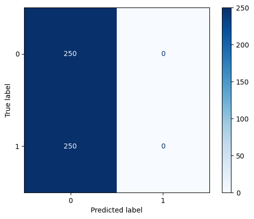
print("Confusion Matrix for Dummy Classifier:")
print(cm_dummy)

Confusion Matrix for Dummy Classifier:
[[250   0]
 [250   0]]

# Visualize the confusion matrix
_ = ConfusionMatrixDisplay.from_estimator(
    dummy,
    X_test,
    y_test,
    cmap=plt.cm.Blues
)

# Calculate test metrics for dummy
accuracy = accuracy_score(y_test, y_pred_dummy)
recall = recall_score(y_test, y_pred_dummy)
precision = precision_score(y_test, y_pred_dummy, zero_division=0)
f1 = f1_score(y_test, y_pred_dummy)
balanced_accuracy = balanced_accuracy_score(y_test, y_pred_dummy)

# Print test metrics for dummy
print(f"Accuracy: {accuracy:.2f}")
print(f"Recall: {recall:.2f}")
print(f"Precision: {precision:.2f}")
print(f"F1 Score: {f1:.2f}")
print(f"Balanced Accuracy: {balanced_accuracy:.2f}")

Accuracy: 0.50
Recall: 0.00
Precision: 0.00
F1 Score: 0.00
Balanced Accuracy: 0.50

# Calculate the confusion matrix for the logistic regression model
cm_lr = confusion_matrix(y_test, y_pred_lr)
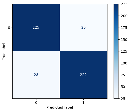
print("Confusion Matrix for Logistic Regression Model:")
print(cm_lr)

Confusion Matrix for Logistic Regression Model:
[[225  25]
 [ 28 222]]

# Visualize the confusion matrix
_ = ConfusionMatrixDisplay.from_estimator(
    lr,
    X_test,
    y_test,
    cmap=plt.cm.Blues
)

# Calculate test metrics for logistic
accuracy = accuracy_score(y_test, y_pred_lr)
recall = recall_score(y_test, y_pred_lr)
precision = precision_score(y_test, y_pred_lr, zero_division=0)
f1 = f1_score(y_test, y_pred_lr)
balanced_accuracy = balanced_accuracy_score(y_test, y_pred_lr)

# Print test metrics for logistic
print(f"Accuracy: {accuracy:.2f}")
print(f"Recall: {recall:.2f}")
print(f"Precision: {precision:.2f}")
print(f"F1 Score: {f1:.2f}")
print(f"Balanced Accuracy: {balanced_accuracy:.2f}")

Accuracy: 0.89
Recall: 0.89
Precision: 0.90
F1 Score: 0.89
Balanced Accuracy: 0.89

# Make predictions with the logistic model with a higher threshold
y_prob_lr = lr.predict_proba(X_test)
y_pred_lr_070 = np.where(y_prob_lr[:, 1] > 0.70, 1, 0)

# Calculate test metrics for logistic, with 0.70 threshold
accuracy = accuracy_score(y_test, y_pred_lr_070)
recall = recall_score(y_test, y_pred_lr_070)
precision = precision_score(y_test, y_pred_lr_070, zero_division=0)
f1 = f1_score(y_test, y_pred_lr_070)
balanced_accuracy = balanced_accuracy_score(y_test, y_pred_lr_070)

# Print test metrics for logistic, with 0.70 threshold
print(f"Accuracy: {accuracy:.2f}")
print(f"Recall: {recall:.2f}")
print(f"Precision: {precision:.2f}")
print(f"F1 Score: {f1:.2f}")
print(f"Balanced Accuracy: {balanced_accuracy:.2f}")

Accuracy: 0.89
Recall: 0.82
Precision: 0.94
F1 Score: 0.88
Balanced Accuracy: 0.89

Imbalanced Data

# Generate an imbalanced classification dataset
X_train, y_train = make_classification(n_samples=500, n_features=10, weights=[0.95, 0.05], random_state=42)
X_test, y_test = make_classification(n_samples=500, n_features=10, weights=[0.95, 0.05], random_state=42)

# Print the number of samples in each class
print("Class 0 samples:", sum(y_train == 0))
print("Class 1 samples:", sum(y_train == 1))

Class 0 samples: 473
Class 1 samples: 27

# Fit logistic regression with no class weights
lr_none = LogisticRegression(max_iter=1000)
lr_none.fit(X_train, y_train)

# Fit logistic regression with balanced class weights
lr_balanced = LogisticRegression(class_weight='balanced', max_iter=1000)
lr_balanced.fit(X_train, y_train)

LogisticRegression(class_weight='balanced', max_iter=1000)

In a Jupyter environment, please rerun this cell to show the HTML representation or trust the notebook.
On GitHub, the HTML representation is unable to render, please try loading this page with nbviewer.org.

# Generate predicted labels for the test data using the logistic regression models
y_pred_lr_none = lr_none.predict(X_test)
y_pred_lr_balanced = lr_balanced.predict(X_test)

# Visualize the confusion matrix
_ = ConfusionMatrixDisplay.from_estimator(
    lr_none,
    X_test,
    y_test,
    cmap=plt.cm.Blues
)

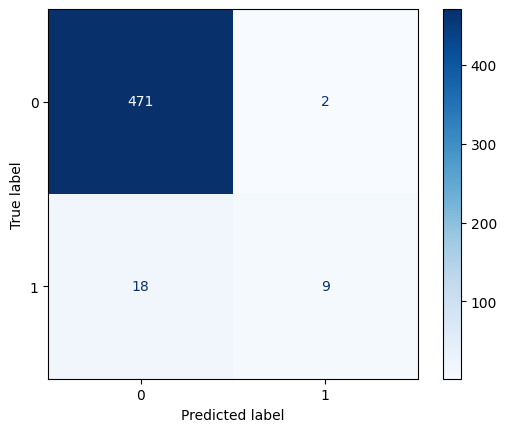
# Calculate test metrics for logistic, no weights
accuracy = accuracy_score(y_test, y_pred_lr_none)
recall = recall_score(y_test, y_pred_lr_none)
precision = precision_score(y_test, y_pred_lr_none, zero_division=0)
f1 = f1_score(y_test, y_pred_lr_none)
balanced_accuracy = balanced_accuracy_score(y_test, y_pred_lr_none)

# Print test metrics for logistic, no weights
print(f"Accuracy: {accuracy:.2f}")
print(f"Recall: {recall:.2f}")
print(f"Precision: {precision:.2f}")
print(f"F1 Score: {f1:.2f}")
print(f"Balanced Accuracy: {balanced_accuracy:.2f}")

Accuracy: 0.96
Recall: 0.33
Precision: 0.82
F1 Score: 0.47
Balanced Accuracy: 0.66

# Visualize the confusion matrix
_ = ConfusionMatrixDisplay.from_estimator(
    lr_balanced,
    X_test,
    y_test,
    cmap=plt.cm.Blues
)

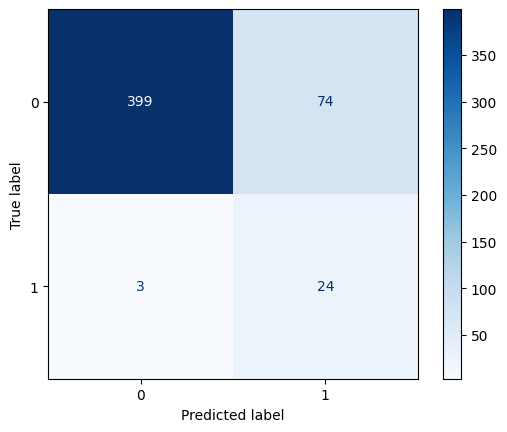
# Calculate test metrics for logistic, balanced weights
accuracy = accuracy_score(y_test, y_pred_lr_balanced)
recall = recall_score(y_test, y_pred_lr_balanced)
precision = precision_score(y_test, y_pred_lr_balanced, zero_division=0)
f1 = f1_score(y_test, y_pred_lr_balanced)
balanced_accuracy = balanced_accuracy_score(y_test, y_pred_lr_balanced)

# Print test metrics for logistic, balanced weights
print(f"Accuracy: {accuracy:.2f}")
print(f"Recall: {recall:.2f}")
print(f"Precision: {precision:.2f}")
print(f"F1 Score: {f1:.2f}")
print(f"Balanced Accuracy: {balanced_accuracy:.2f}")

Accuracy: 0.85
Recall: 0.89
Precision: 0.24
F1 Score: 0.38
Balanced Accuracy: 0.87

Spam Data

• UCI Machine Learning Repository: Spambase

column_names = [
    "word_freq_make",
    "word_freq_address",
    "word_freq_all",
    "word_freq_3d",
    "word_freq_our",
    "word_freq_over",
    "word_freq_remove",
    "word_freq_internet",
    "word_freq_order",
    "word_freq_mail",
    "word_freq_receive",
    "word_freq_will",
    "word_freq_people",
    "word_freq_report",
    "word_freq_addresses",
    "word_freq_free",
    "word_freq_business",
    "word_freq_email",
    "word_freq_you",
    "word_freq_credit",
    "word_freq_your",
    "word_freq_font",
    "word_freq_000",
    "word_freq_money",
    "word_freq_hp",
    "word_freq_hpl",
    "word_freq_george",
    "word_freq_650",
    "word_freq_lab",
    "word_freq_labs",
    "word_freq_telnet",
    "word_freq_857",
    "word_freq_data",
    "word_freq_415",
    "word_freq_85",
    "word_freq_technology",
    "word_freq_1999",
    "word_freq_parts",
    "word_freq_pm",
    "word_freq_direct",
    "word_freq_cs",
    "word_freq_meeting",
    "word_freq_original",
    "word_freq_project",
    "word_freq_re",
    "word_freq_edu",
    "word_freq_table",
    "word_freq_conference",
    "char_freq_semicolon",
    "char_freq_parenthesis",
    "char_freq_bracket",
    "char_freq_exclamation",
    "char_freq_dollar",
    "char_freq_hash",
    "capital_run_length_average",
    "capital_run_length_longest",
    "capital_run_length_total",
    "spam",
]

spam_data = pd.read_csv("https://www.cs307.org/notes/week-09/data/spambase.csv")

# Split the data into training and testing sets
X_train, X_test, y_train, y_test = train_test_split(
    spam_data.drop(columns=["spam"]),
    spam_data["spam"],
    test_size=0.2,
    random_state=42
)

# define scoring metrics
scoring = {
    "accuracy": make_scorer(accuracy_score),
    "recall": make_scorer(recall_score),
    "precision": make_scorer(precision_score, zero_division=0),
    "f1": make_scorer(f1_score),
}

# setup random forest
rf_param_grid = {
    "n_estimators": [100, 250],
    "max_depth": [1, 10, 50],
    "class_weight": [{0: 2, 1: 1}, {0: 1, 1: 1}, {0: 1, 1: 2}],
}
rf = RandomForestClassifier(random_state=42)

# setup grid search objects
rf_grid = GridSearchCV(rf, rf_param_grid, cv=3, scoring=scoring, refit="f1", n_jobs=-1, verbose=1)

# fit models via grid search
rf_grid.fit(X_train, y_train)

Fitting 3 folds for each of 18 candidates, totalling 54 fits

GridSearchCV(cv=3, estimator=RandomForestClassifier(random_state=42), n_jobs=-1,
             param_grid={'class_weight': [{0: 2, 1: 1}, {0: 1, 1: 1},
                                          {0: 1, 1: 2}],
                         'max_depth': [1, 10, 50], 'n_estimators': [100, 250]},
             refit='f1',
             scoring={'accuracy': make_scorer(accuracy_score),
                      'f1': make_scorer(f1_score),
                      'precision': make_scorer(precision_score, zero_division=0),
                      'recall': make_scorer(recall_score)},
             verbose=1)

In a Jupyter environment, please rerun this cell to show the HTML representation or trust the notebook.
On GitHub, the HTML representation is unable to render, please try loading this page with nbviewer.org.

# define a function to print metric scores for the best estimator
def print_metric_scores(grid, metric):
    cv_results = grid.cv_results_
    best_index = grid.best_index_
    mean_score = cv_results[f"mean_test_{metric}"][best_index]
    std_score = cv_results[f"std_test_{metric}"][best_index]
    print(f"CV {metric} (mean ± std): {mean_score:.3f} ± {std_score:.3f}")

print(f"Best parameters: {rf_grid.best_params_}")
print("")
print_metric_scores(rf_grid, "accuracy")
print_metric_scores(rf_grid, "recall")
print_metric_scores(rf_grid, "precision")
print_metric_scores(rf_grid, "f1")

Best parameters: {'class_weight': {0: 1, 1: 1}, 'max_depth': 50, 'n_estimators': 250}

CV accuracy (mean ± std): 0.949 ± 0.007
CV recall (mean ± std): 0.921 ± 0.005
CV precision (mean ± std): 0.946 ± 0.016
CV f1 (mean ± std): 0.933 ± 0.008

# predict on test data
y_pred = rf_grid.predict(X_test)

# calculate test accuracy
test_accuracy = accuracy_score(y_test, y_pred)
print("")
print(f"Test Accuracy: {test_accuracy}")

Test Accuracy: 0.9587404994571118

# calculate test precision and recall
precision = precision_score(y_test, y_pred)
recall = recall_score(y_test, y_pred)
print(f"Test Precision: {precision}")
print(f"Test Recall: {recall}")

Test Precision: 0.9782608695652174
Test Recall: 0.9230769230769231

# calculate test confusion matrix
cm = confusion_matrix(y_test, y_pred)

# extract TP, FP, TN, FN
tn, fp, fn, tp = cm.ravel()
print("")
print(f"Test True Positives: {tp}")
print(f"Test True Negatives: {tn}")
print(f"Test False Positives: {fp}")
print(f"Test False Negatives: {fn}")

Test True Positives: 360
Test True Negatives: 523
Test False Positives: 8
Test False Negatives: 30