CS 307: Week 10

# Basics
import numpy as np
import pandas as pd
import matplotlib.pyplot as plt
import seaborn as sns
import warnings

# Probability
from scipy.stats import multivariate_normal

# Machine Learning
from sklearn.preprocessing import StandardScaler
from sklearn.discriminant_analysis import LinearDiscriminantAnalysis
from sklearn.discriminant_analysis import QuadraticDiscriminantAnalysis
from sklearn.naive_bayes import GaussianNB

# Classification Metrics
from sklearn.metrics import accuracy_score, confusion_matrix
from sklearn.metrics import ConfusionMatrixDisplay

# Deal with pandas versus seaborn issues
warnings.simplefilter(action="ignore", category=FutureWarning)

Some Bayes Theorem

Given priors:

• \(\pi_A = 0.20\)
• \(\pi_B = 0.50\)
• \(\pi_C = 0.30\)

And likelihoods:

• \(X \mid Y = A \sim N(\mu = 2, \sigma = 1)\)
• \(X \mid Y = B \sim N(\mu = 3, \sigma = 2)\)
• \(X \mid Y = C \sim N(\mu = 4, \sigma = 1)\)

Calculate posteriors:

• \(P(Y = A \mid X = 3.4)\)
• \(P(Y = B \mid X = 3.4)\)
• \(P(Y = C \mid X = 3.4)\)

import numpy as np
from scipy.stats import norm
import matplotlib.pyplot as plt

x = np.linspace(-2, 8, 1000)
mu = [2, 3, 4]
sigma = [1, 2, 1]

fig, axs = plt.subplots(1, 2, figsize=(12, 5))

for i in range(3):
    y = norm.pdf(x, loc=mu[i], scale=sigma[i])
    axs[0].plot(x, y, label=f"Y={chr(65+i)}", linewidth=2)

axs[0].axvline(x=3.4, color="red", linestyle="--")
axs[0].set_xlabel("X")
axs[0].set_ylabel("Density")
axs[0].grid(color="lightgrey", linestyle="--")
axs[0].set_title("Likelihoods")
axs[0].legend()

priors = [0.20, 0.50, 0.30]

z = []
for i in range(len(x)):
    z.append(np.sum(priors * norm.pdf(x[i], loc=mu, scale=sigma)))

for i in range(3):
    y = priors[i] * norm.pdf(x, loc=mu[i], scale=sigma[i])
    axs[1].plot(x, y / z, label=f"Y={chr(65+i)}", linewidth=2)

axs[1].axvline(x=3.4, color="red", linestyle="--")
axs[1].set_xlabel("X")
axs[1].set_ylabel("Density")
axs[1].grid(color="lightgrey", linestyle="--")
axs[1].set_title("Posteriors")
axs[1].legend()

plt.show()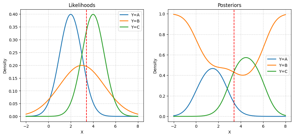

import numpy as np
from scipy.stats import norm

priors = [0.20, 0.50, 0.30]
likelihoods = norm.pdf(x=3.4, loc=[2, 3, 4], scale=[1, 2, 1])
priors * likelihoods / (np.sum(priors * likelihoods))

array([0.13152821, 0.42938969, 0.43908211])

• \(P(Y = A \mid X = 3.7) = 0.13152821\)
• \(P(Y = B \mid X = 3.7) = 0.42938969\)
• \(P(Y = C \mid X = 3.7) = 0.43908211\)

Generative Models

\[ p_k(\boldsymbol{x}) = P(Y = k \mid \boldsymbol{X} = \boldsymbol{x}) = \frac{\pi_k \cdot f_k(\boldsymbol{x})}{\sum_{g = 1}^{G} \pi_g \cdot f_g(\boldsymbol{x})} \]

Helper Functions

def make_plot(mu1, cov1, mu2, cov2):
    # Create two multivariate normal distributions
    dist1 = multivariate_normal(mu1, cov1)
    dist2 = multivariate_normal(mu2, cov2)

    # Generate random samples from each distribution
    samples1 = dist1.rvs(size=100)
    samples2 = dist2.rvs(size=100)

    # Change color maps for scatter plot
    cmap1 = plt.get_cmap("Blues")
    cmap2 = plt.get_cmap("Oranges")

    # Plot true distributions
    x_min = np.min([np.min(samples1[:, 0]), np.min(samples2[:, 0])]) - 1
    x_max = np.max([np.max(samples1[:, 0]), np.max(samples2[:, 0])]) + 1
    y_min = np.min([np.min(samples1[:, 1]), np.min(samples2[:, 1])]) - 1
    y_max = np.max([np.max(samples1[:, 1]), np.max(samples2[:, 1])]) + 1
    x, y = np.mgrid[x_min:x_max:0.01, y_min:y_max:0.01]
    pos = np.empty(x.shape + (2,))
    pos[:, :, 0] = x
    pos[:, :, 1] = y
    fig, ax = plt.subplots(1, 2, figsize=(10, 5))
    ax[0].contourf(x, y, dist1.pdf(pos), cmap="Blues")
    ax[0].contour(x, y, dist1.pdf(pos), colors="k")
    ax[0].contourf(x, y, dist2.pdf(pos), cmap="Oranges", alpha=0.5)
    ax[0].contour(x, y, dist2.pdf(pos), colors="k")
    ax[0].grid(color="lightgrey", linestyle="--")
    ax[0].set_title("True Distribution")
    ax[1].scatter(samples1[:, 0], samples1[:, 1], color=cmap1(0.5))
    ax[1].scatter(samples2[:, 0], samples2[:, 1], color=cmap2(0.5))
    ax[1].set_title("Sampled Data")
    ax[1].grid(color="lightgrey", linestyle="--")
    ax[0].set_xlim(x_min, x_max)
    ax[0].set_ylim(y_min, y_max)
    ax[1].set_xlim(x_min, x_max)
    ax[1].set_ylim(y_min, y_max)
    plt.show()

# Create mean (mu) and covariance (cov) arrays
def create_params(mu_1, mu_2, sigma_1, sigma_2, corr):
    # Create mean vector
    mu = np.array([mu_1, mu_2])
    # Calculate covariance matrix
    cov = np.array([[sigma_1**2, corr * sigma_1 * sigma_2], [corr * sigma_1 * sigma_2, sigma_2**2]])
    # Return both
    return mu, cov

# Print parameter information
def print_setup_parameter_info(mu1, cov1, mu2, cov2):
    print("Mean X when Y = Blue:", mu1)
    print("Covariance of X when Y = Blue:", "\n", cov1)
    print("Mean X when Y = Orange:", mu2)
    print("Covariance of X when Y = Orange:", "\n", cov2)

Linear Discriminant Analysis (LDA)

Linear Discriminant Analysis, LDA, assumes that the features are multivariate normal conditioned on the target classes. Importantly, LDA assumes the same covariance (shape) within each class.

\[ \boldsymbol{X} \mid Y = k \sim N(\boldsymbol{\mu}_k, \boldsymbol\Sigma) \]

\[ \boldsymbol\Sigma = \boldsymbol\Sigma_1 = \boldsymbol\Sigma_2 = \cdots = \boldsymbol\Sigma_G \]

# Make a two-class LDA setup
mu1, cov1 = create_params(0, 0, 1, 1, 0.5)
mu2, cov2 = create_params(2, 2, 1, 1, 0.5)
print_setup_parameter_info(mu1, cov1, mu2, cov2)

Mean X when Y = Blue: [0 0]
Covariance of X when Y = Blue: 
 [[1.  0.5]
 [0.5 1. ]]
Mean X when Y = Orange: [2 2]
Covariance of X when Y = Orange: 
 [[1.  0.5]
 [0.5 1. ]]

# Plot it!
make_plot(mu1, cov1, mu2, cov2)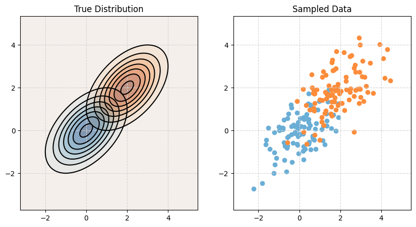

Quadratic Discriminant Analysis (QDA)

Quadratic Discriminant Analysis, QDA, also assumes that the features are multivariate normal conditioned on the target classes. However, unlike LDA, QDA makes fewer assumptions on the covariances (shapes). QDA allows the covariance to be completely different within each class.

\[ \boldsymbol X \mid Y = k \sim N(\boldsymbol\mu_k, \boldsymbol\Sigma_k) \]

# Make a two-class QDA setup
mu1, cov1 = create_params(0, 0, 2, 1, 0.5)
mu2, cov2 = create_params(2, 2, 1, 0.5, -0.5)
print_setup_parameter_info(mu1, cov1, mu2, cov2)

Mean X when Y = Blue: [0 0]
Covariance of X when Y = Blue: 
 [[4. 1.]
 [1. 1.]]
Mean X when Y = Orange: [2 2]
Covariance of X when Y = Orange: 
 [[ 1.   -0.25]
 [-0.25  0.25]]

# Plot it!
make_plot(mu1, cov1, mu2, cov2)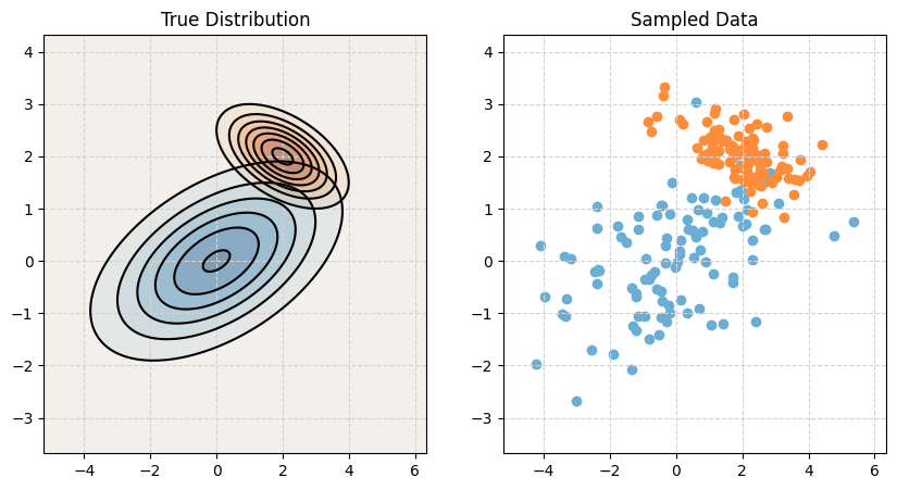

Naive Bayes (NB)

Naive Bayes comes in many forms. With only numeric features, it often assumes a multivariate normal conditioned on the target classes, but a very specific multivariate normal.

\[ {\boldsymbol X} \mid Y = k \sim N(\boldsymbol\mu_k, \boldsymbol\Sigma_k) \]

Naive Bayes assumes that the features \(X_1, X_2, \ldots, X_p\) are independent given \(Y = k\). This is the “naive” part of naive Bayes. The Bayes part is nothing new. Since \(X_1, X_2, \ldots, X_p\) are assumed independent, each \(\boldsymbol\Sigma_k\) is diagonal, that is, we assume no correlation between features. Independence implies zero correlation.

\[ \boldsymbol\Sigma_k = \begin{bmatrix} \sigma_{1}^2 & 0 & \cdots & 0 \\ 0 & \ddots & \ddots & \vdots \\ \vdots & \ddots & \ddots & 0 \\ 0 & \cdots & 0 & \sigma_{p}^2 \\ \end{bmatrix} \]

This will allow us to write the (joint) likelihood as a product of univariate distributions. In this case, the product of univariate normal distributions instead of a (joint) multivariate distribution.

\[ f_k(\boldsymbol x) = \prod_{j = 1}^{p} f_{kj}(\boldsymbol x_j) \]

Here, \(f_{kj}(\boldsymbol x_j)\) is the density for the \(j\)-th feature conditioned on the \(k\)-th class. Notice that there is a \(\sigma_{kj}\) for each feature for each class.

\[ f_{kj}(\boldsymbol x_j) = \frac{1}{\sigma_{kj}\sqrt{2\pi}}\exp\left[-\frac{1}{2}\left(\frac{x_j - \mu_{kj}}{\sigma_{kj}}\right)^2\right] \]

When \(p = 1\), this version of naive Bayes is equivalent to QDA.

# Make a two-class NB setup
mu1, cov1 = create_params(0, 0, 2, 1, 0)
mu2, cov2 = create_params(2, 2, 1, 0.5, 0)
print_setup_parameter_info(mu1, cov1, mu2, cov2)

Mean X when Y = Blue: [0 0]
Covariance of X when Y = Blue: 
 [[4 0]
 [0 1]]
Mean X when Y = Orange: [2 2]
Covariance of X when Y = Orange: 
 [[1.   0.  ]
 [0.   0.25]]

# Plot it!
make_plot(mu1, cov1, mu2, cov2)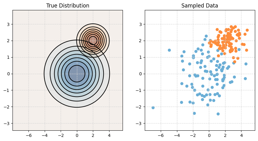

Generative Models with sklearn

# Function to generate data according to LDA, QDA, or NB
def generate_data(n1, n2, n3, mu1, mu2, mu3, cov1, cov2, cov3):
    # Generate data for class A
    data1 = np.random.multivariate_normal(mu1, cov1, n1)
    labels1 = np.repeat("A", n1)

    # Generate data for class B
    data2 = np.random.multivariate_normal(mu2, cov2, n2)
    labels2 = np.repeat("B", n2)

    # Generate data for class C
    data3 = np.random.multivariate_normal(mu3, cov3, n3)
    labels3 = np.repeat("C", n3)

    # Combine data and labels
    data = np.concatenate((data1, data2, data3))
    labels = np.concatenate((labels1, labels2, labels3))

    # Make X and y
    X = pd.DataFrame(data, columns=["x1", "x2"])
    y = pd.Series(labels)

    return X, y

# Setup sample sizes
n1 = 500
n2 = 500
n3 = 500

# Setup parameters
mu1, cov1 = create_params(0, 0, 2, 1, 0.5)
mu2, cov2 = create_params(2, 2, 1, 2, -0.5)
mu3, cov3 = create_params(0, 2, 1, 1, 0.5)

# Generate train and test data
X_train, y_train = generate_data(n1, n2, n3, mu1, mu2, mu3, cov1, cov2, cov3)
X_test, y_test = generate_data(n1, n2, n3, mu1, mu2, mu3, cov1, cov2, cov3)

# Plot the train data
p = sns.jointplot(x="x1", y="x2", data=X_train, hue=y_train, space=0)
p.fig.suptitle("Simulated Train Data", y=1.01)
p.ax_joint.grid(True)
p.fig.set_size_inches(8, 8)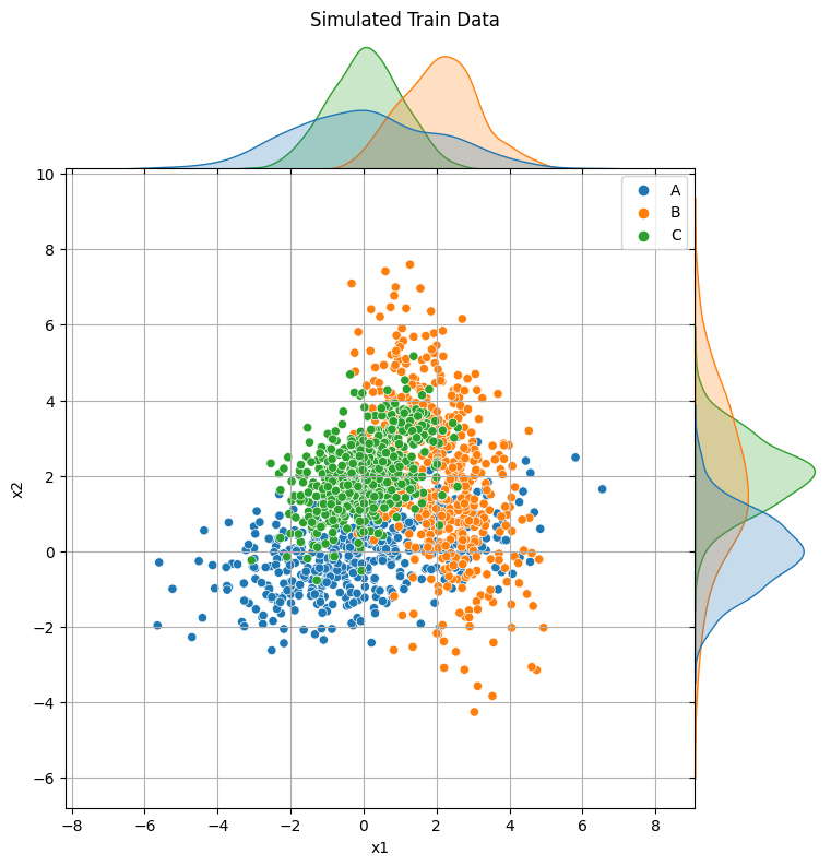

# Gaussian Naive Bayes
gnb = GaussianNB()
gnb.fit(X_train, y_train)
y_pred = gnb.predict(X_test)
accuracy = accuracy_score(y_test, y_pred)
print("Gaussian NB, Test Accuracy:", accuracy)

# Linear Discriminant Analysis
lda = LinearDiscriminantAnalysis(store_covariance=True)
lda.fit(X_train, y_train)
y_pred = lda.predict(X_test)
accuracy = accuracy_score(y_test, y_pred)
print("LDA, Test Accuracy:", accuracy)

# Quadratic Discriminant Analysis
qda = QuadraticDiscriminantAnalysis(store_covariance=True)
qda.fit(X_train, y_train)
y_pred = qda.predict(X_test)
accuracy = accuracy_score(y_test, y_pred)
print("QDA, Test Accuracy:", accuracy)

Gaussian NB, Test Accuracy: 0.7466666666666667
LDA, Test Accuracy: 0.688
QDA, Test Accuracy: 0.758

print("Classes:", gnb.classes_)
print("Feature names:", gnb.feature_names_in_)
print("NB, Estimated Class Priors:", gnb.class_prior_)
print("NB, Estimated Mean of each feature per class:", "\n", gnb.theta_)
print("NB, Estimated Variance of each feature per class:", "\n", gnb.var_)

Classes: ['A' 'B' 'C']
Feature names: ['x1' 'x2']
NB, Estimated Class Priors: [0.33333333 0.33333333 0.33333333]
NB, Estimated Mean of each feature per class: 
 [[4.01566160e-02 2.38873059e-05]
 [2.08143224e+00 1.97557520e+00]
 [3.66427998e-02 2.06823633e+00]]
NB, Estimated Variance of each feature per class: 
 [[4.04651343 0.97403523]
 [1.07528142 4.16455559]
 [0.95628049 0.86020391]]

print("Classes:", qda.classes_)
print("Feature names:", qda.feature_names_in_)
print("QDA, Estimated Class Priors:", qda.priors_)
print("QDA, Estimated Mean of each feature per class:", "\n", qda.means_)
print("QDA, Estimated Covariance Matrix of each feature per class:")
qda.covariance_

Classes: ['A' 'B' 'C']
Feature names: ['x1' 'x2']
QDA, Estimated Class Priors: [0.33333333 0.33333333 0.33333333]
QDA, Estimated Mean of each feature per class: 
 [[4.01566160e-02 2.38873059e-05]
 [2.08143224e+00 1.97557520e+00]
 [3.66427998e-02 2.06823633e+00]]
QDA, Estimated Covariance Matrix of each feature per class:

[array([[4.05462268, 0.92459548],
        [0.92459548, 0.9759872 ]]),
 array([[ 1.07743629, -0.94226649],
        [-0.94226649,  4.17290139]]),
 array([[0.95819688, 0.41460533],
        [0.41460533, 0.86192776]])]

Effect of Scaling

# Scale the X data
scaler = StandardScaler()
X_train_scaled = scaler.fit_transform(X_train)
X_test_scaled = scaler.transform(X_test)

p = sns.jointplot(x="x1", y="x2", data=pd.DataFrame(X_train_scaled, columns=["x1", "x2"]), hue=y_train, space=0)
p.fig.suptitle("Simulated Train Data, Scaled", y=1.01)
p.ax_joint.grid(True)
p.fig.set_size_inches(8, 8)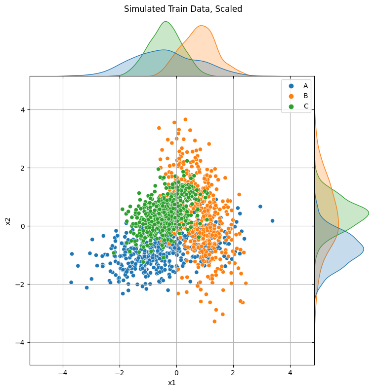

# Fit NB model again
gnbs = GaussianNB()
gnbs.fit(X_train_scaled, y_train)
y_pred = gnbs.predict(X_test_scaled)

# Calculate accuracy
accuracy = accuracy_score(y_test, y_pred)
print("Accuracy:", accuracy)

Accuracy: 0.7466666666666667

# Check estimated probabilities
gnb.predict_proba(X_test) == gnbs.predict_proba(X_test_scaled)
np.allclose(gnb.predict_proba(X_test), gnbs.predict_proba(X_test_scaled))

True

print("Classes:", gnbs.classes_)
print("NB, Estimated Class Priors:", gnbs.class_prior_)
print("NB, Estimated Mean of each feature per class:", "\n", gnbs.theta_)
print("NB, Estimated Variance of each feature per class:", "\n", gnbs.var_)

Classes: ['A' 'B' 'C']
NB, Estimated Class Priors: [0.33333333 0.33333333 0.33333333]
NB, Estimated Mean of each feature per class: 
 [[-0.39523727 -0.79023671]
 [ 0.79251912  0.36795645]
 [-0.39728185  0.42228026]]
NB, Estimated Variance of each feature per class: 
 [[1.37003745 0.3347804 ]
 [0.36406053 1.43137695]
 [0.3237701  0.29565605]]

Priors

# Setup sample sizes
n1_train = 500
n2_train = 300
n3_train = 700
n1_test = 500
n2_test = 500
n3_test = 500

# Setup parameters
mu1, cov1 = create_params(0, 0, 2, 1, 0.5)
mu2, cov2 = create_params(2, 2, 1, 2, -0.5)
mu3, cov3 = create_params(0, 2, 1, 1, 0.5)

# Generate train and test data
X_train, y_train = generate_data(n1_train, n2_train, n3_train, mu1, mu2, mu3, cov1, cov2, cov3)
X_test, y_test = generate_data(n1_test, n2_test, n3_test, mu1, mu2, mu3, cov1, cov2, cov3)

# Quadratic Discriminant Analysis, Estimated Prior
qda = QuadraticDiscriminantAnalysis(store_covariance=True)
qda.fit(X_train, y_train)
y_pred = qda.predict(X_test)
accuracy = accuracy_score(y_test, y_pred)
print("QDA, Test Accuracy:", accuracy)

QDA, Test Accuracy: 0.756

# Quadratic Discriminant Analysis, Specified Prior
qda = QuadraticDiscriminantAnalysis(store_covariance=True, priors=[0.33, 0.33, 0.33])
qda.fit(X_train, y_train)
y_pred = qda.predict(X_test)
accuracy = accuracy_score(y_test, y_pred)
print("QDA, Test Accuracy:", accuracy)

QDA, Test Accuracy: 0.764

Penguins

from palmerpenguins import load_penguins
import pandas as pd
from sklearn.model_selection import train_test_split
from sklearn.pipeline import Pipeline
from sklearn.compose import ColumnTransformer
from sklearn.impute import SimpleImputer
from sklearn.preprocessing import StandardScaler, OneHotEncoder
from sklearn.svm import SVC
from sklearn.model_selection import GridSearchCV

# Load the dataset
penguins = load_penguins()

# Convert to pandas dataframe
df = pd.DataFrame(penguins)

# Print the first 5 rows of the dataframe
df.head()

	species	island	bill_length_mm	bill_depth_mm	flipper_length_mm	body_mass_g	sex	year
0	Adelie	Torgersen	39.1	18.7	181.0	3750.0	male	2007
1	Adelie	Torgersen	39.5	17.4	186.0	3800.0	female	2007
2	Adelie	Torgersen	40.3	18.0	195.0	3250.0	female	2007
3	Adelie	Torgersen	NaN	NaN	NaN	NaN	NaN	2007
4	Adelie	Torgersen	36.7	19.3	193.0	3450.0	female	2007

# Create X and y
df = df.drop("year", axis=1)
X = df.drop("species", axis=1)
y = df["species"]

# Split the data into training and testing sets
X_train, X_test, y_train, y_test = train_test_split(X, y, test_size=0.2, random_state=42)

# Print the shapes of the resulting dataframes
print("X_train shape:", X_train.shape)
print("y_train shape:", y_train.shape)
print("X_test shape:", X_test.shape)
print("y_test shape:", y_test.shape)

X_train shape: (275, 6)
y_train shape: (275,)
X_test shape: (69, 6)
y_test shape: (69,)

X_train

	island	bill_length_mm	bill_depth_mm	flipper_length_mm	body_mass_g	sex
66	Biscoe	35.5	16.2	195.0	3350.0	female
229	Biscoe	51.1	16.3	220.0	6000.0	male
7	Torgersen	39.2	19.6	195.0	4675.0	male
140	Dream	40.2	17.1	193.0	3400.0	female
323	Dream	49.0	19.6	212.0	4300.0	male
...	...	...	...	...	...	...
188	Biscoe	42.6	13.7	213.0	4950.0	female
71	Torgersen	39.7	18.4	190.0	3900.0	male
106	Biscoe	38.6	17.2	199.0	3750.0	female
270	Biscoe	47.2	13.7	214.0	4925.0	female
102	Biscoe	37.7	16.0	183.0	3075.0	female

275 rows × 6 columns

y_train

66        Adelie
229       Gentoo
7         Adelie
140       Adelie
323    Chinstrap
         ...    
188       Gentoo
71        Adelie
106       Adelie
270       Gentoo
102       Adelie
Name: species, Length: 275, dtype: object

# Define the numeric features
numeric_features = ["bill_length_mm", "bill_depth_mm", "flipper_length_mm", "body_mass_g"]

# Define the categorical features
categorical_features = ["sex", "island"]

# Define the column transformer
preprocessor = ColumnTransformer(
    transformers=[
        ("num", StandardScaler(), numeric_features),
        ("cat", OneHotEncoder(), categorical_features),
    ]
)

# Define the full pipeline
pipe = Pipeline([("preprocessor", preprocessor), ("imputer", SimpleImputer()), ("classifier", SVC())])

# Define the parameter grid
param_grid = {
    "imputer__strategy": ["mean", "median"],
    "classifier__C": [0.1, 1, 10],
    "classifier__kernel": ["linear", "rbf"],
}

# Define the grid search
grid = GridSearchCV(pipe, param_grid=param_grid, cv=5, verbose=1)

# Fit the grid search to the training data
grid.fit(X_train, y_train)

# Print the best parameters and score
print("Best parameters:", grid.best_params_)
print("Best score:", grid.best_score_)

Fitting 5 folds for each of 12 candidates, totalling 60 fits
Best parameters: {'classifier__C': 0.1, 'classifier__kernel': 'linear', 'imputer__strategy': 'mean'}
Best score: 0.9927272727272728

grid

GridSearchCV(cv=5,
             estimator=Pipeline(steps=[('preprocessor',
                                        ColumnTransformer(transformers=[('num',
                                                                         StandardScaler(),
                                                                         ['bill_length_mm',
                                                                          'bill_depth_mm',
                                                                          'flipper_length_mm',
                                                                          'body_mass_g']),
                                                                        ('cat',
                                                                         OneHotEncoder(),
                                                                         ['sex',
                                                                          'island'])])),
                                       ('imputer', SimpleImputer()),
                                       ('classifier', SVC())]),
             param_grid={'classifier__C': [0.1, 1, 10],
                         'classifier__kernel': ['linear', 'rbf'],
                         'imputer__strategy': ['mean', 'median']},
             verbose=1)

In a Jupyter environment, please rerun this cell to show the HTML representation or trust the notebook.
On GitHub, the HTML representation is unable to render, please try loading this page with nbviewer.org.

One-Hot Encoding

X_train_cat = X_train[categorical_features]
X_train_cat.to_numpy()[:10]

array([['female', 'Biscoe'],
       ['male', 'Biscoe'],
       ['male', 'Torgersen'],
       ['female', 'Dream'],
       ['male', 'Dream'],
       ['male', 'Dream'],
       ['male', 'Dream'],
       ['female', 'Torgersen'],
       ['female', 'Dream'],
       ['female', 'Dream']], dtype=object)

ohe = OneHotEncoder(sparse_output=False)
ohe.fit(X_train_cat)
ohe.fit_transform(X_train_cat)

array([[1., 0., 0., 1., 0., 0.],
       [0., 1., 0., 1., 0., 0.],
       [0., 1., 0., 0., 0., 1.],
       ...,
       [1., 0., 0., 1., 0., 0.],
       [1., 0., 0., 1., 0., 0.],
       [1., 0., 0., 1., 0., 0.]])

de = OneHotEncoder(sparse_output=False, drop="first")
de.fit(X_train_cat)
de.fit_transform(X_train_cat)

array([[0., 0., 0., 0.],
       [1., 0., 0., 0.],
       [1., 0., 0., 1.],
       ...,
       [0., 0., 0., 0.],
       [0., 0., 0., 0.],
       [0., 0., 0., 0.]])

Imputation

X_train_num = X_train[numeric_features]
X_train_num_nan = X_train_num[X_train.isna().any(axis=1)]
X_train_num_nan.to_numpy()

array([[  47.3,   13.8,  216. , 4725. ],
       [   nan,    nan,    nan,    nan],
       [  37.8,   17.1,  186. , 3300. ],
       [  44.5,   14.3,  216. , 4100. ],
       [  44.5,   15.7,  217. , 4875. ],
       [  46.2,   14.4,  214. , 4650. ],
       [  37.5,   18.9,  179. , 2975. ],
       [  37.8,   17.3,  180. , 3700. ],
       [  34.1,   18.1,  193. , 3475. ]])

imp = SimpleImputer()
imp.fit(X_train_num)
imp.fit_transform(X_train_num_nan)

array([[  47.3   ,   13.8   ,  216.    , 4725.    ],
       [  41.2125,   16.2   ,  200.125 , 3975.    ],
       [  37.8   ,   17.1   ,  186.    , 3300.    ],
       [  44.5   ,   14.3   ,  216.    , 4100.    ],
       [  44.5   ,   15.7   ,  217.    , 4875.    ],
       [  46.2   ,   14.4   ,  214.    , 4650.    ],
       [  37.5   ,   18.9   ,  179.    , 2975.    ],
       [  37.8   ,   17.3   ,  180.    , 3700.    ],
       [  34.1   ,   18.1   ,  193.    , 3475.    ]])