# standard imports
import matplotlib.pyplot as plt
import numpy as np
import random

# sklearn imports
from sklearn.datasets import load_digits
from sklearn.metrics import accuracy_score
from sklearn.model_selection import train_test_split
from sklearn.ensemble import RandomForestClassifier
from sklearn.neural_network import MLPClassifier
from sklearn.metrics import ConfusionMatrixDisplay

# pytorch imports
import torch
from torch import nn
from torch.utils.data import DataLoader
from torchvision import datasets
from torchvision.transforms import ToTensor
from torchsummary import summaryCS 307: Week 12
# %pip install torch
# %pip install torchvision
# %pip install torchsummary
MNIST with Random Forest
digits = load_digits()digits{'data': array([[ 0., 0., 5., ..., 0., 0., 0.],
[ 0., 0., 0., ..., 10., 0., 0.],
[ 0., 0., 0., ..., 16., 9., 0.],
...,
[ 0., 0., 1., ..., 6., 0., 0.],
[ 0., 0., 2., ..., 12., 0., 0.],
[ 0., 0., 10., ..., 12., 1., 0.]]),
'target': array([0, 1, 2, ..., 8, 9, 8]),
'frame': None,
'feature_names': ['pixel_0_0',
'pixel_0_1',
'pixel_0_2',
'pixel_0_3',
'pixel_0_4',
'pixel_0_5',
'pixel_0_6',
'pixel_0_7',
'pixel_1_0',
'pixel_1_1',
'pixel_1_2',
'pixel_1_3',
'pixel_1_4',
'pixel_1_5',
'pixel_1_6',
'pixel_1_7',
'pixel_2_0',
'pixel_2_1',
'pixel_2_2',
'pixel_2_3',
'pixel_2_4',
'pixel_2_5',
'pixel_2_6',
'pixel_2_7',
'pixel_3_0',
'pixel_3_1',
'pixel_3_2',
'pixel_3_3',
'pixel_3_4',
'pixel_3_5',
'pixel_3_6',
'pixel_3_7',
'pixel_4_0',
'pixel_4_1',
'pixel_4_2',
'pixel_4_3',
'pixel_4_4',
'pixel_4_5',
'pixel_4_6',
'pixel_4_7',
'pixel_5_0',
'pixel_5_1',
'pixel_5_2',
'pixel_5_3',
'pixel_5_4',
'pixel_5_5',
'pixel_5_6',
'pixel_5_7',
'pixel_6_0',
'pixel_6_1',
'pixel_6_2',
'pixel_6_3',
'pixel_6_4',
'pixel_6_5',
'pixel_6_6',
'pixel_6_7',
'pixel_7_0',
'pixel_7_1',
'pixel_7_2',
'pixel_7_3',
'pixel_7_4',
'pixel_7_5',
'pixel_7_6',
'pixel_7_7'],
'target_names': array([0, 1, 2, 3, 4, 5, 6, 7, 8, 9]),
'images': array([[[ 0., 0., 5., ..., 1., 0., 0.],
[ 0., 0., 13., ..., 15., 5., 0.],
[ 0., 3., 15., ..., 11., 8., 0.],
...,
[ 0., 4., 11., ..., 12., 7., 0.],
[ 0., 2., 14., ..., 12., 0., 0.],
[ 0., 0., 6., ..., 0., 0., 0.]],
[[ 0., 0., 0., ..., 5., 0., 0.],
[ 0., 0., 0., ..., 9., 0., 0.],
[ 0., 0., 3., ..., 6., 0., 0.],
...,
[ 0., 0., 1., ..., 6., 0., 0.],
[ 0., 0., 1., ..., 6., 0., 0.],
[ 0., 0., 0., ..., 10., 0., 0.]],
[[ 0., 0., 0., ..., 12., 0., 0.],
[ 0., 0., 3., ..., 14., 0., 0.],
[ 0., 0., 8., ..., 16., 0., 0.],
...,
[ 0., 9., 16., ..., 0., 0., 0.],
[ 0., 3., 13., ..., 11., 5., 0.],
[ 0., 0., 0., ..., 16., 9., 0.]],
...,
[[ 0., 0., 1., ..., 1., 0., 0.],
[ 0., 0., 13., ..., 2., 1., 0.],
[ 0., 0., 16., ..., 16., 5., 0.],
...,
[ 0., 0., 16., ..., 15., 0., 0.],
[ 0., 0., 15., ..., 16., 0., 0.],
[ 0., 0., 2., ..., 6., 0., 0.]],
[[ 0., 0., 2., ..., 0., 0., 0.],
[ 0., 0., 14., ..., 15., 1., 0.],
[ 0., 4., 16., ..., 16., 7., 0.],
...,
[ 0., 0., 0., ..., 16., 2., 0.],
[ 0., 0., 4., ..., 16., 2., 0.],
[ 0., 0., 5., ..., 12., 0., 0.]],
[[ 0., 0., 10., ..., 1., 0., 0.],
[ 0., 2., 16., ..., 1., 0., 0.],
[ 0., 0., 15., ..., 15., 0., 0.],
...,
[ 0., 4., 16., ..., 16., 6., 0.],
[ 0., 8., 16., ..., 16., 8., 0.],
[ 0., 1., 8., ..., 12., 1., 0.]]]),
'DESCR': ".. _digits_dataset:\n\nOptical recognition of handwritten digits dataset\n--------------------------------------------------\n\n**Data Set Characteristics:**\n\n :Number of Instances: 1797\n :Number of Attributes: 64\n :Attribute Information: 8x8 image of integer pixels in the range 0..16.\n :Missing Attribute Values: None\n :Creator: E. Alpaydin (alpaydin '@' boun.edu.tr)\n :Date: July; 1998\n\nThis is a copy of the test set of the UCI ML hand-written digits datasets\nhttps://archive.ics.uci.edu/ml/datasets/Optical+Recognition+of+Handwritten+Digits\n\nThe data set contains images of hand-written digits: 10 classes where\neach class refers to a digit.\n\nPreprocessing programs made available by NIST were used to extract\nnormalized bitmaps of handwritten digits from a preprinted form. From a\ntotal of 43 people, 30 contributed to the training set and different 13\nto the test set. 32x32 bitmaps are divided into nonoverlapping blocks of\n4x4 and the number of on pixels are counted in each block. This generates\nan input matrix of 8x8 where each element is an integer in the range\n0..16. This reduces dimensionality and gives invariance to small\ndistortions.\n\nFor info on NIST preprocessing routines, see M. D. Garris, J. L. Blue, G.\nT. Candela, D. L. Dimmick, J. Geist, P. J. Grother, S. A. Janet, and C.\nL. Wilson, NIST Form-Based Handprint Recognition System, NISTIR 5469,\n1994.\n\n|details-start|\n**References**\n|details-split|\n\n- C. Kaynak (1995) Methods of Combining Multiple Classifiers and Their\n Applications to Handwritten Digit Recognition, MSc Thesis, Institute of\n Graduate Studies in Science and Engineering, Bogazici University.\n- E. Alpaydin, C. Kaynak (1998) Cascading Classifiers, Kybernetika.\n- Ken Tang and Ponnuthurai N. Suganthan and Xi Yao and A. Kai Qin.\n Linear dimensionalityreduction using relevance weighted LDA. School of\n Electrical and Electronic Engineering Nanyang Technological University.\n 2005.\n- Claudio Gentile. A New Approximate Maximal Margin Classification\n Algorithm. NIPS. 2000.\n\n|details-end|"}digits.images[0]array([[ 0., 0., 5., 13., 9., 1., 0., 0.],
[ 0., 0., 13., 15., 10., 15., 5., 0.],
[ 0., 3., 15., 2., 0., 11., 8., 0.],
[ 0., 4., 12., 0., 0., 8., 8., 0.],
[ 0., 5., 8., 0., 0., 9., 8., 0.],
[ 0., 4., 11., 0., 1., 12., 7., 0.],
[ 0., 2., 14., 5., 10., 12., 0., 0.],
[ 0., 0., 6., 13., 10., 0., 0., 0.]])digits.targetarray([0, 1, 2, ..., 8, 9, 8])_, axes = plt.subplots(nrows=10, ncols=20, figsize=(10, 5))
for i in range(10):
digit_examples = digits.images[digits.target == i]
for j in range(20):
axes[i][j].set_axis_off()
axes[i][j].imshow(digit_examples[j], cmap=plt.cm.gray_r)
plt.show()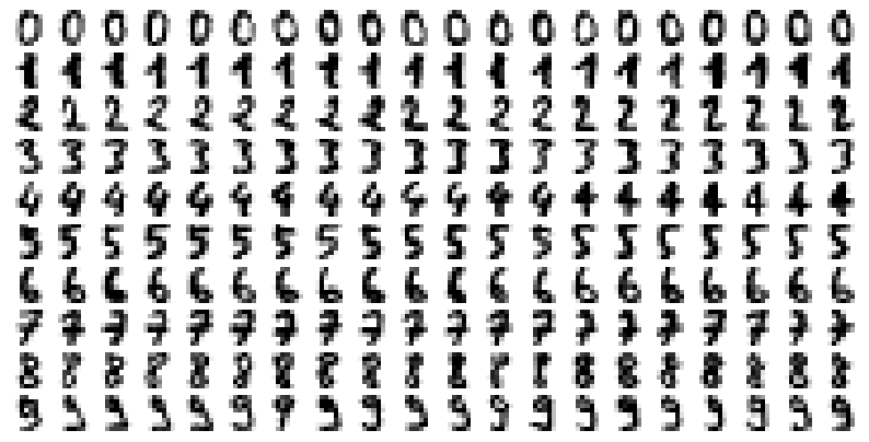
# flatten the images
n_samples = len(digits.images)
data = digits.images.reshape((n_samples, -1))
data[0]
array([ 0., 0., 5., 13., 9., 1., 0., 0., 0., 0., 13., 15., 10.,
15., 5., 0., 0., 3., 15., 2., 0., 11., 8., 0., 0., 4.,
12., 0., 0., 8., 8., 0., 0., 5., 8., 0., 0., 9., 8.,
0., 0., 4., 11., 0., 1., 12., 7., 0., 0., 2., 14., 5.,
10., 12., 0., 0., 0., 0., 6., 13., 10., 0., 0., 0.])# Create a classifier: a random forest classifier
clf = RandomForestClassifier()# Split data into 50% train and 50% test subsets
X_train, X_test, y_train, y_test = train_test_split(
data, digits.target, test_size=0.5, random_state=1
)
# Learn the digits on the train subset
clf.fit(X_train, y_train)
# Predict the value of the digit on the test subset
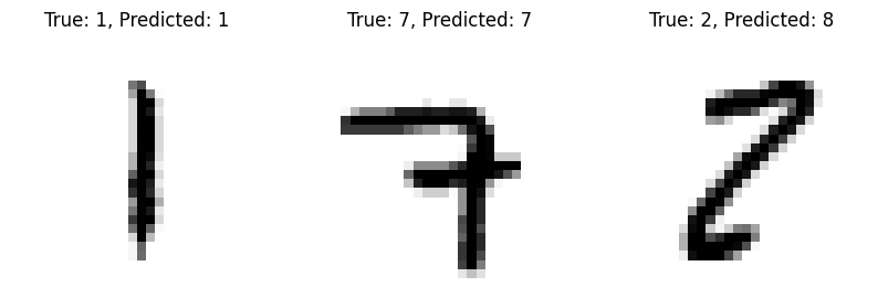
predicted = clf.predict(X_test)n_test = len(predicted)
idx = random.sample(range(0, n_test), 4)
_, axes = plt.subplots(nrows=1, ncols=4, figsize=(10, 3))
for ax, image, true_label, predicted_label in zip(axes, X_test[idx], y_test[idx], predicted[idx]):
ax.set_axis_off()
image = image.reshape(8, 8)
ax.imshow(image, cmap=plt.cm.gray_r)
ax.set_title(f"True: {true_label}, Predicted: {predicted_label}")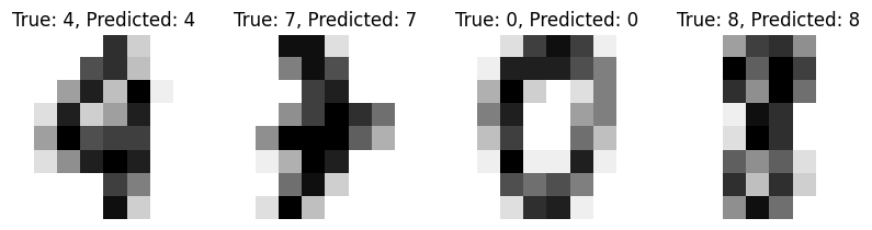
disp = ConfusionMatrixDisplay.from_predictions(y_test, predicted)
disp.figure_.suptitle("Confusion Matrix")
print(f"Confusion matrix:\n{disp.confusion_matrix}")

plt.show()
Confusion matrix:
[[ 81 0 0 0 2 0 0 0 0 0]
[ 0 92 0 0 0 1 0 0 0 0]
[ 0 0 85 0 0 0 0 0 0 0]
[ 0 0 0 94 0 0 0 2 2 0]
[ 0 0 0 0 100 0 0 0 0 0]
[ 0 0 0 0 1 78 1 0 1 0]
[ 0 1 0 0 0 0 87 0 0 0]
[ 0 0 0 0 0 0 0 88 0 1]
[ 0 0 1 0 0 0 0 0 80 0]
[ 0 1 0 2 0 5 0 2 1 90]]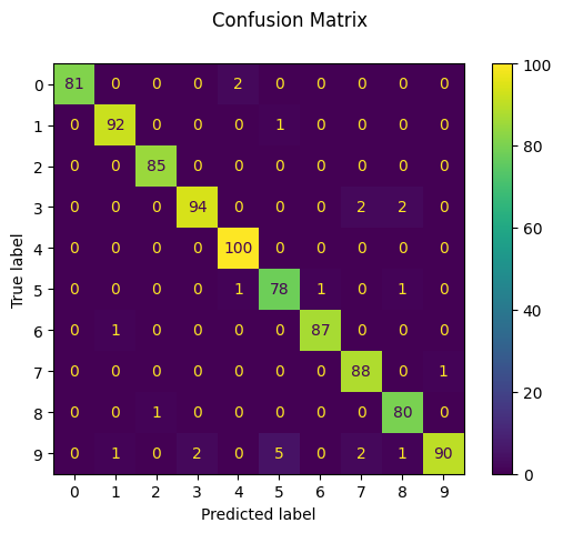
accuracy = accuracy_score(y_test, predicted)
print(f"Accuracy: {accuracy}")
Accuracy: 0.9733036707452726MNIST with a Neural Network in sklearn
# Create a classifier: a MLP classifier
clf = MLPClassifier(
    hidden_layer_sizes=(512, 512, 512, 256, 128, 10),
    max_iter=1000,
    alpha=0.003,
    random_state=42,
    verbose=True,
)

# Learn the digits on the train subset
clf.fit(X_train, y_train)

# Predict the value of the digit on the test subset
predicted = clf.predict(X_test)

# Print the accuracy score
accuracy = accuracy_score(y_test, predicted)
print(f"Accuracy: {accuracy}")
Iteration 1, loss = 2.36251904
Iteration 2, loss = 1.62066731
Iteration 3, loss = 1.14226786
Iteration 4, loss = 0.86670278
Iteration 5, loss = 0.69921045
Iteration 6, loss = 0.57739401
Iteration 7, loss = 0.49723736
Iteration 8, loss = 0.45362170
Iteration 9, loss = 0.40136902
Iteration 10, loss = 0.36432217
Iteration 11, loss = 0.33676894
Iteration 12, loss = 0.31571457
Iteration 13, loss = 0.29946901
Iteration 14, loss = 0.28576926
Iteration 15, loss = 0.27574156
Iteration 16, loss = 0.26992495
Iteration 17, loss = 0.26917527
Iteration 18, loss = 0.26789323
Iteration 19, loss = 0.26811930
Iteration 20, loss = 0.26476725
Iteration 21, loss = 0.26369207
Iteration 22, loss = 0.26130162
Iteration 23, loss = 0.25763350
Iteration 24, loss = 0.25515783
Iteration 25, loss = 0.25535490
Iteration 26, loss = 0.25103766
Iteration 27, loss = 0.25985071
Iteration 28, loss = 0.26210301
Iteration 29, loss = 0.27255595
Iteration 30, loss = 0.26786620
Iteration 31, loss = 0.26879423
Iteration 32, loss = 0.26683657
Iteration 33, loss = 0.26367676
Iteration 34, loss = 0.25193371
Iteration 35, loss = 0.24592936
Iteration 36, loss = 0.24579529
Iteration 37, loss = 0.24093999
Iteration 38, loss = 0.24051345
Iteration 39, loss = 0.23892965
Iteration 40, loss = 0.23999483
Iteration 41, loss = 0.23897436
Iteration 42, loss = 0.23874734
Iteration 43, loss = 0.23427278
Iteration 44, loss = 0.23424035
Iteration 45, loss = 0.23196924
Iteration 46, loss = 0.23041228
Iteration 47, loss = 0.22826713
Iteration 48, loss = 0.22601849
Iteration 49, loss = 0.22366596
Iteration 50, loss = 0.22145363
Iteration 51, loss = 0.21883771
Iteration 52, loss = 0.21595303
Iteration 53, loss = 0.21283027
Iteration 54, loss = 0.20946229
Iteration 55, loss = 0.20592629
Iteration 56, loss = 0.20346813
Iteration 57, loss = 0.19789268
Iteration 58, loss = 0.19334121
Iteration 59, loss = 0.18814408
Iteration 60, loss = 0.18303965
Iteration 61, loss = 0.17695626
Iteration 62, loss = 0.17097079
Iteration 63, loss = 0.16338590
Iteration 64, loss = 0.15561319
Iteration 65, loss = 0.14700656
Iteration 66, loss = 0.13740347
Iteration 67, loss = 0.12580355
Iteration 68, loss = 0.11302574
Iteration 69, loss = 0.09676645
Iteration 70, loss = 0.07605584
Iteration 71, loss = 0.05099887
Iteration 72, loss = 0.02775913
Iteration 73, loss = 0.01962240
Iteration 74, loss = 0.01760788
Iteration 75, loss = 0.03705301
Iteration 76, loss = 0.07079593
Iteration 77, loss = 0.11612643
Iteration 78, loss = 0.12089772
Iteration 79, loss = 0.07980162
Iteration 80, loss = 0.06225297
Iteration 81, loss = 0.03408364
Iteration 82, loss = 0.02340592
Iteration 83, loss = 0.01841710
Iteration 84, loss = 0.01606490
Iteration 85, loss = 0.01283442
Iteration 86, loss = 0.01239670
Iteration 87, loss = 0.01216325
Iteration 88, loss = 0.01192471
Iteration 89, loss = 0.01177482
Iteration 90, loss = 0.01169969
Iteration 91, loss = 0.01165434
Iteration 92, loss = 0.01162437
Iteration 93, loss = 0.01160123
Iteration 94, loss = 0.01158161
Iteration 95, loss = 0.01156299
Iteration 96, loss = 0.01154546
Iteration 97, loss = 0.01152992
Iteration 98, loss = 0.01151456
Iteration 99, loss = 0.01150046
Iteration 100, loss = 0.01148661
Training loss did not improve more than tol=0.000100 for 10 consecutive epochs. Stopping.
Accuracy: 0.9688542825361512MNIST with a Neural Network in pytorch
# Download training data from open datasets.
training_data = datasets.MNIST(
    root="data",
    train=True,
    download=True,
    transform=ToTensor(),
)

# Download test data from open datasets.
test_data = datasets.MNIST(
    root="data",
    train=False,
    download=True,
    transform=ToTensor(),
)
batch_size = 64
# Create data loaders.
train_dataloader = DataLoader(training_data, batch_size=batch_size)
test_dataloader = DataLoader(test_data, batch_size=batch_size)
for X, y in test_dataloader:
print(f"Shape of X [N, C, H, W]: {X.shape}")
print(f"Shape of y: {y.shape} {y.dtype}")
breakShape of X [N, C, H, W]: torch.Size([64, 1, 28, 28])
Shape of y: torch.Size([64]) torch.int64# Get cpu, gpu or mps device for training.
device = (
"cuda" if torch.cuda.is_available() else "mps" if torch.backends.mps.is_available() else "cpu"
)
print(f"Using {device} device")Using mps device# Define model
class NeuralNetwork(nn.Module):
def __init__(self):
super().__init__()
self.flatten = nn.Flatten()
self.linear_relu_stack = nn.Sequential(
nn.Linear(28 * 28, 512),
nn.ReLU(),
nn.Linear(512, 512),
nn.ReLU(),
nn.Linear(512, 10),
)
def forward(self, x):
x = self.flatten(x)
logits = self.linear_relu_stack(x)
return logits
model = NeuralNetwork().to(device)
print(model)NeuralNetwork(
(flatten): Flatten(start_dim=1, end_dim=-1)
(linear_relu_stack): Sequential(
(0): Linear(in_features=784, out_features=512, bias=True)
(1): ReLU()
(2): Linear(in_features=512, out_features=512, bias=True)
(3): ReLU()
(4): Linear(in_features=512, out_features=10, bias=True)
)
)loss_fn = nn.CrossEntropyLoss()
optimizer = torch.optim.SGD(model.parameters(), lr=1e-3)def train(dataloader, model, loss_fn, optimizer):
size = len(dataloader.dataset)
model.train()
for batch, (X, y) in enumerate(dataloader):
X, y = X.to(device), y.to(device)
# Compute prediction error
pred = model(X)
loss = loss_fn(pred, y)
# Backpropagation
loss.backward()
optimizer.step()
optimizer.zero_grad()
if batch % 100 == 0:
loss, current = loss.item(), (batch + 1) * len(X)
print(f"loss: {loss:>7f} [{current:>5d}/{size:>5d}]")def test(dataloader, model, loss_fn):
size = len(dataloader.dataset)
num_batches = len(dataloader)
model.eval()
test_loss, correct = 0, 0
with torch.no_grad():
for X, y in dataloader:
X, y = X.to(device), y.to(device)
pred = model(X)
test_loss += loss_fn(pred, y).item()
correct += (pred.argmax(1) == y).type(torch.float).sum().item()
test_loss /= num_batches
correct /= size
print(f"Test Error: \n Accuracy: {(100*correct):>0.1f}%, Avg loss: {test_loss:>8f} \n")epochs = 15
for t in range(epochs):
print(f"Epoch {t+1}\n-------------------------------")
train(train_dataloader, model, loss_fn, optimizer)
test(test_dataloader, model, loss_fn)
print("Done!")Epoch 1
-------------------------------
loss: 2.306658 [ 64/60000]
loss: 2.290079 [ 6464/60000]
loss: 2.282270 [12864/60000]
loss: 2.287214 [19264/60000]
loss: 2.285212 [25664/60000]
loss: 2.275597 [32064/60000]
loss: 2.271847 [38464/60000]
loss: 2.270402 [44864/60000]
loss: 2.264636 [51264/60000]
loss: 2.255980 [57664/60000]
Test Error:
Accuracy: 51.0%, Avg loss: 2.252304
Epoch 2
-------------------------------
loss: 2.256287 [ 64/60000]
loss: 2.239189 [ 6464/60000]
loss: 2.238762 [12864/60000]
loss: 2.217500 [19264/60000]
loss: 2.231100 [25664/60000]
loss: 2.221864 [32064/60000]
loss: 2.202883 [38464/60000]
loss: 2.220133 [44864/60000]
loss: 2.193508 [51264/60000]
loss: 2.179165 [57664/60000]
Test Error:
Accuracy: 64.3%, Avg loss: 2.178734
Epoch 3
-------------------------------
loss: 2.182662 [ 64/60000]
loss: 2.161872 [ 6464/60000]
loss: 2.171301 [12864/60000]
loss: 2.112587 [19264/60000]
loss: 2.143860 [25664/60000]
loss: 2.133374 [32064/60000]
loss: 2.091750 [38464/60000]
loss: 2.132885 [44864/60000]
loss: 2.075600 [51264/60000]
loss: 2.049700 [57664/60000]
Test Error:
Accuracy: 66.7%, Avg loss: 2.051171
Epoch 4
-------------------------------
loss: 2.056093 [ 64/60000]
loss: 2.024727 [ 6464/60000]
loss: 2.049628 [12864/60000]
loss: 1.934100 [19264/60000]
loss: 1.986609 [25664/60000]
loss: 1.973067 [32064/60000]
loss: 1.899264 [38464/60000]
loss: 1.974741 [44864/60000]
loss: 1.875368 [51264/60000]
loss: 1.830791 [57664/60000]
Test Error:
Accuracy: 67.9%, Avg loss: 1.830845
Epoch 5
-------------------------------
loss: 1.839905 [ 64/60000]
loss: 1.788181 [ 6464/60000]
loss: 1.835950 [12864/60000]
loss: 1.657672 [19264/60000]
loss: 1.723784 [25664/60000]
loss: 1.704309 [32064/60000]
loss: 1.605233 [38464/60000]
loss: 1.726989 [44864/60000]
loss: 1.585339 [51264/60000]
loss: 1.527164 [57664/60000]
Test Error:
Accuracy: 71.8%, Avg loss: 1.519282
Epoch 6
-------------------------------
loss: 1.542019 [ 64/60000]
loss: 1.460990 [ 6464/60000]
loss: 1.533268 [12864/60000]
loss: 1.334707 [19264/60000]
loss: 1.390277 [25664/60000]
loss: 1.366181 [32064/60000]
loss: 1.269149 [38464/60000]
loss: 1.435188 [44864/60000]
loss: 1.284903 [51264/60000]
loss: 1.224249 [57664/60000]
Test Error:
Accuracy: 77.0%, Avg loss: 1.206172
Epoch 7
-------------------------------
loss: 1.250360 [ 64/60000]
loss: 1.147594 [ 6464/60000]
loss: 1.228017 [12864/60000]
loss: 1.062284 [19264/60000]
loss: 1.098954 [25664/60000]
loss: 1.074481 [32064/60000]
loss: 0.992385 [38464/60000]
loss: 1.176954 [44864/60000]
loss: 1.055590 [51264/60000]
loss: 0.993100 [57664/60000]
Test Error:
Accuracy: 80.3%, Avg loss: 0.969658
Epoch 8
-------------------------------
loss: 1.033129 [ 64/60000]
loss: 0.916886 [ 6464/60000]
loss: 0.989789 [12864/60000]
loss: 0.870227 [19264/60000]
loss: 0.897028 [25664/60000]
loss: 0.871840 [32064/60000]
loss: 0.800789 [38464/60000]
loss: 0.984963 [44864/60000]
loss: 0.901598 [51264/60000]
loss: 0.838112 [57664/60000]
Test Error:
Accuracy: 82.3%, Avg loss: 0.809710
Epoch 9
-------------------------------
loss: 0.883999 [ 64/60000]
loss: 0.760413 [ 6464/60000]
loss: 0.822977 [12864/60000]
loss: 0.741897 [19264/60000]
loss: 0.762487 [25664/60000]
loss: 0.738000 [32064/60000]
loss: 0.670728 [38464/60000]
loss: 0.850335 [44864/60000]
loss: 0.797148 [51264/60000]
loss: 0.736822 [57664/60000]
Test Error:
Accuracy: 83.8%, Avg loss: 0.701605
Epoch 10
-------------------------------
loss: 0.780015 [ 64/60000]
loss: 0.653056 [ 6464/60000]
loss: 0.707583 [12864/60000]
loss: 0.655317 [19264/60000]
loss: 0.669251 [25664/60000]
loss: 0.648301 [32064/60000]
loss: 0.579144 [38464/60000]
loss: 0.756160 [44864/60000]
loss: 0.721586 [51264/60000]
loss: 0.669211 [57664/60000]
Test Error:
Accuracy: 84.8%, Avg loss: 0.625850
Epoch 11
-------------------------------
loss: 0.704309 [ 64/60000]
loss: 0.576131 [ 6464/60000]
loss: 0.625620 [12864/60000]
loss: 0.595386 [19264/60000]
loss: 0.601341 [25664/60000]
loss: 0.585813 [32064/60000]
loss: 0.511969 [38464/60000]
loss: 0.689301 [44864/60000]
loss: 0.663925 [51264/60000]
loss: 0.622493 [57664/60000]
Test Error:
Accuracy: 85.7%, Avg loss: 0.570618
Epoch 12
-------------------------------
loss: 0.646772 [ 64/60000]
loss: 0.518795 [ 6464/60000]
loss: 0.565227 [12864/60000]
loss: 0.552369 [19264/60000]
loss: 0.549810 [25664/60000]
loss: 0.541016 [32064/60000]
loss: 0.461181 [38464/60000]
loss: 0.640739 [44864/60000]
loss: 0.618332 [51264/60000]
loss: 0.589068 [57664/60000]
Test Error:
Accuracy: 86.5%, Avg loss: 0.528853
Epoch 13
-------------------------------
loss: 0.601402 [ 64/60000]
loss: 0.474660 [ 6464/60000]
loss: 0.518948 [12864/60000]
loss: 0.520428 [19264/60000]
loss: 0.509435 [25664/60000]
loss: 0.507891 [32064/60000]
loss: 0.421873 [38464/60000]
loss: 0.604481 [44864/60000]
loss: 0.581360 [51264/60000]
loss: 0.564317 [57664/60000]
Test Error:
Accuracy: 87.0%, Avg loss: 0.496268
Epoch 14
-------------------------------
loss: 0.564502 [ 64/60000]
loss: 0.439818 [ 6464/60000]
loss: 0.482281 [12864/60000]
loss: 0.495910 [19264/60000]
loss: 0.476937 [25664/60000]
loss: 0.482654 [32064/60000]
loss: 0.390765 [38464/60000]
loss: 0.576522 [44864/60000]
loss: 0.550761 [51264/60000]
loss: 0.545336 [57664/60000]
Test Error:
Accuracy: 87.6%, Avg loss: 0.470175
Epoch 15
-------------------------------
loss: 0.533683 [ 64/60000]
loss: 0.411910 [ 6464/60000]
loss: 0.452353 [12864/60000]
loss: 0.476562 [19264/60000]
loss: 0.450214 [25664/60000]
loss: 0.462852 [32064/60000]
loss: 0.365653 [38464/60000]
loss: 0.554290 [44864/60000]
loss: 0.525229 [51264/60000]
loss: 0.530438 [57664/60000]
Test Error:
Accuracy: 88.0%, Avg loss: 0.448842
Done!torch.save(model.state_dict(), "model.pth")
print("Saved PyTorch Model State to model.pth")Saved PyTorch Model State to model.pth# Get a batch of training data
batch = next(iter(train_dataloader))
images, labels = batch
# Plot the first three images in the batch
fig, axs = plt.subplots(1, 3, figsize=(10, 5))
for i in range(3):
axs[i].set_axis_off()
axs[i].imshow(images[i].squeeze(), cmap=plt.cm.gray_r)
axs[i].set_title(f"Label: {labels[i]}")
plt.show()
n_test = len(test_data)
idx = random.sample(range(0, n_test), 10)

_, axes = plt.subplots(nrows=1, ncols=3, figsize=(10, 3))
for ax, idx in zip(axes, idx):
    image, label = test_data[idx]
    image = image.unsqueeze(0)
    with torch.no_grad():
        model.eval()
        output = model(image.to(device))
        predicted = output.argmax(1).item()
    ax.set_axis_off()
    image = image.squeeze()
    ax.imshow(image, cmap=plt.cm.gray_r)
    ax.set_title(f"True: {label}, Predicted: {predicted}")
plt.show()